

In his weblog submit, Enrique Pinzon mentioned the right way to carry out regression once we don’t wish to make any assumptions about practical kind—use the npregress command. He concluded by asking and answering just a few questions concerning the outcomes utilizing the margins and marginsplot instructions.
Not too long ago, I’ve been interested by all of the several types of questions that we may reply utilizing margins after nonparametric regression, or actually after any kind of regression. margins and marginsplot are highly effective instruments for exploring the outcomes of a mannequin and drawing many sorts of inferences. On this submit, I’ll present you the right way to ask and reply very particular questions and the right way to discover all the response floor primarily based on the outcomes of your nonparametric regression.
The dataset that we’ll use consists of three covariates—steady variables x1 and x2 and categorical variable a with three ranges. If you need to comply with alongside, you should utilize these knowledge by typing use http://www.stata.com/customers/kmacdonald/weblog/npblog.
Let’s first match our mannequin.
. npregress kernel y x1 x2 i.a, vce(boot, rep(10) seed(111))
(working npregress on estimation pattern)

Bootstrap replications (10)
----+--- 1 ---+--- 2 ---+--- 3 ---+--- 4 ---+--- 5
..........

Bandwidth
------------------------------------
             |      Imply     Impact
-------------+----------------------
          x1 |  .4795422   1.150255
          x2 |  .7305017    1.75222
           a |  .3872428   .3872428
------------------------------------

Native-linear regression                    Variety of obs      =          1,497
Steady kernel : epanechnikov           E(Kernel obs)      =            524
Discrete kernel   : liracine               R-squared          =         0.8762
Bandwidth         : cross validation
------------------------------------------------------------------------------
             |   Noticed   Bootstrap                          Percentile
           y |   Estimate   Std. Err.      z    P>|z|     [95% Conf. Interval]
-------------+----------------------------------------------------------------
Imply         |
           y |   15.64238   .3282016    47.66   0.000     15.17505    16.38781
-------------+----------------------------------------------------------------
Impact       |
          x1 |   3.472485   .2614388    13.28   0.000     2.895202    3.846091
          x2 |   4.143544   .2003619    20.68   0.000     3.830656    4.441306
             |
           a |
   (2 vs 1)  |   1.512241   .2082431     7.26   0.000     .9880627    1.717007
   (3 vs 1)  |  -10.23723   .2679278   -38.21   0.000     -10.6352   -9.715858
------------------------------------------------------------------------------
Observe: Impact estimates are averages of derivatives for steady covariates
      and averages of contrasts for issue covariates.
Enrique mentioned interpretation of those ends in his weblog, so I can’t deal with it right here. I ought to, nevertheless, level out that as a result of my purpose is to point out you the right way to use margins, I used solely 10 bootstrap replications (a ridiculously small quantity) when estimating commonplace errors. In actual analysis, you will surely wish to use extra replications each with the npregress command and the margins instructions that comply with.
The npregress output consists of estimates of the consequences of x1, x2, and the degrees of a on our consequence, however these estimates are in all probability not sufficient to reply among the necessary questions that we wish to handle in our analysis.
Under, I’ll first present you how one can discover the nonlinear response floor—the anticipated worth of y at totally different mixtures of x1, x2, and a. As an illustration, suppose your consequence variable is the response to a drug, and also you wish to know the anticipated worth for a feminine whose weight is 150 kilos and whose ldl cholesterol degree is 220 milligrams per deciliter. What about for a male with the identical traits? How do these expectations change throughout a variety of weights and levels of cholesterol?
I may even exhibit the right way to reply questions on inhabitants averages, counterfactuals, remedy results, and extra. These are precisely the kinds of questions that coverage makers ask. How, on common, does a variable have an effect on the inhabitants they’re excited about? As an illustration, suppose your consequence variable is earnings of people of their 20s. What’s the anticipated worth of earnings for this group, the inhabitants common? What’s the anticipated worth if, as a substitute of getting their noticed schooling degree, they have been all highschool graduates? What in the event that they have been all school graduates? What’s the distinction in these values—the impact of school schooling?
These are only a few examples of the kinds of questions that you may reply. I’ll proceed with variable names x1, x2, and a beneath, however you may think about related questions in your analysis.
Exploring the response floor
Let’s begin at the start. We would wish to know the anticipated worth of the end result at one particular level. To get the anticipated worth of y when a=1, x1=2, and x2=5, we are able to kind
. margins 1.a, at(x1=2 x2=5) reps(10)
(working margins on estimation pattern)

Bootstrap replications (10)
----+--- 1 ---+--- 2 ---+--- 3 ---+--- 4 ---+--- 5
..........

Adjusted predictions                            Variety of obs     =      1,497
                                                Replications      =         10

Expression   : imply perform, predict()
at           : x1              =           2
               x2              =           5

------------------------------------------------------------------------------
             |   Noticed   Bootstrap                          Percentile
             |     Margin   Std. Err.      z    P>|z|     [95% Conf. Interval]
-------------+----------------------------------------------------------------
         1.a |   12.66575   .4428049    28.60   0.000     11.57809     13.0897
------------------------------------------------------------------------------
We predict that y=12.7 at this level.
We may consider it at one other level, say, a=2, x1=2, and x2=5.
. margins 2.a, at(x1=2 x2=5) reps(10)
(working margins on estimation pattern)

Bootstrap replications (10)
----+--- 1 ---+--- 2 ---+--- 3 ---+--- 4 ---+--- 5
..........

Adjusted predictions                            Variety of obs     =      1,497
                                                Replications      =         10

Expression   : imply perform, predict()
at           : x1              =           2
               x2              =           5

------------------------------------------------------------------------------
             |   Noticed   Bootstrap                          Percentile
             |     Margin   Std. Err.      z    P>|z|     [95% Conf. Interval]
-------------+----------------------------------------------------------------
         2.a |   14.80935   .6774548    21.86   0.000     13.48154    15.98991
------------------------------------------------------------------------------
With a=2, the anticipated worth of y is now 14.8.
What if our curiosity is within the impact of going from a=1 to a=2 when x1=2 and x2=5? That’s only a distinction—the distinction in our two earlier outcomes. Utilizing the r. distinction operator with margins, we are able to carry out a speculation check of whether or not these two values are the identical.
. margins r(1 2).a, at(x1=2 x2=5) reps(10)
(working margins on estimation pattern)

Bootstrap replications (10)
----+--- 1 ---+--- 2 ---+--- 3 ---+--- 4 ---+--- 5
..........
Contrasts of predictive margins
                                                Variety of obs     =      1,497
                                                Replications      =         10

Expression   : imply perform, predict()
at           : x1              =           2
               x2              =           5

------------------------------------------------
             |         df        chi2     P>chi2
-------------+----------------------------------
           a |          1       27.58     0.0000
------------------------------------------------

--------------------------------------------------------------
             |   Noticed   Bootstrap          Percentile
             |   Distinction   Std. Err.     [95% Conf. Interval]
-------------+------------------------------------------------
           a |
   (2 vs 1)  |   2.143598   .4081472      1.335078    2.523469
--------------------------------------------------------------
The arrogance interval for the distinction doesn’t embody 0. Utilizing a 5% significance degree, we discover that the anticipated worth is considerably totally different for these two factors of curiosity.
However we is perhaps excited about greater than these two factors. Let’s proceed holding x2 to five and have a look at a variety of values for x1. And let’s estimate the anticipated values throughout all three ranges of a. In different phrases, let’s have a look at a slice of the three-d response floor (at x2=5) and study the connection between the opposite two variables.
. margins a, at(x1=(1(1)4) x2=5) reps(10)
(working margins on estimation pattern)

Bootstrap replications (10)
----+--- 1 ---+--- 2 ---+--- 3 ---+--- 4 ---+--- 5
..........

Adjusted predictions                            Variety of obs     =      1,497
                                                Replications      =         10

Expression   : imply perform, predict()

1._at        : x1              =           1
               x2              =           5

2._at        : x1              =           2
               x2              =           5

3._at        : x1              =           3
               x2              =           5

4._at        : x1              =           4
               x2              =           5

------------------------------------------------------------------------------
             |   Noticed   Bootstrap                          Percentile
             |     Margin   Std. Err.      z    P>|z|     [95% Conf. Interval]
-------------+----------------------------------------------------------------
       _at#a |
        1 1  |   9.075231   2.017476     4.50   0.000     5.984868    12.61052
        1 2  |   14.35551   2.488854     5.77   0.000     9.944582    17.73349
        1 3  |  -.2925357   1.499151    -0.20   0.845    -1.991074    2.248606
        2 1  |   12.66575   .3285203    38.55   0.000     11.93955    13.03459
        2 2  |   14.80935   .8713405    17.00   0.000     12.92743    15.75046
        2 3  |    1.82419   .5384259     3.39   0.001     .6331934    2.422084
        3 1  |    17.1207   .2446792    69.97   0.000     16.89714    17.61579
        3 2  |   17.28286   .3536435    48.87   0.000     16.78102    17.89018
        3 3  |     6.2364   .2689665    23.19   0.000     5.695041      6.5686
        4 1  |   21.29851   .1441116   147.79   0.000     21.05866    21.54149
        4 2  |   18.96943   .2000661    94.82   0.000     18.50348    19.24232
        4 3  |   11.45945   .2037134    56.25   0.000     11.05172    11.69403
------------------------------------------------------------------------------
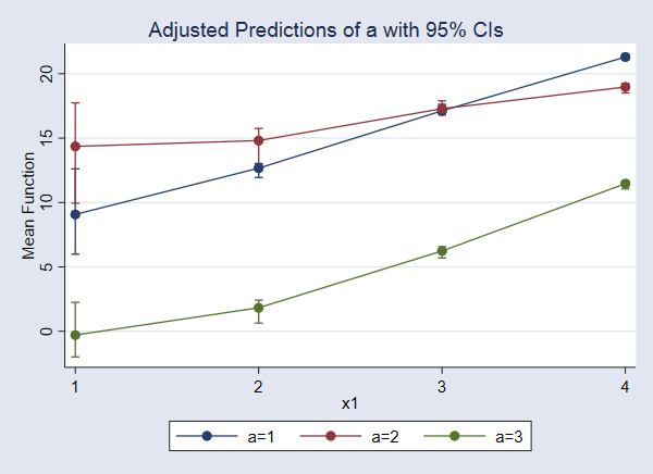
Higher but, let’s plot these values.
. marginsplot
We discover that when x2=5, the anticipated worth of y will increase as x1 will increase, and the anticipated worth is decrease for a=3 than for a=1 and a=2 throughout all ranges of x1.
However is that this sample the identical for different values of x2?
We have now solely three covariates. So we are able to discover all the response floor simply. Let’s have a look at extra slices at different values of x2. Right here’s the command:
. margins a, at(x1=(1(1)4) x2=(2 5 8)) reps(10)
This produces quite a lot of output, so I gained’t present it. However right here is the graph
. marginsplot, bydimension(x2) byopts(cols(3))
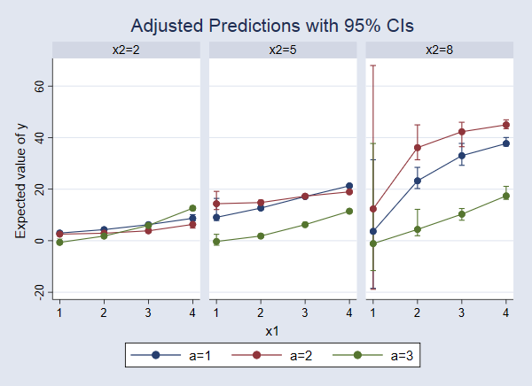
We are able to now see that the response floor adjustments as x2 adjustments. When x2=2, the anticipated worth of y will increase barely as x1 will increase, however there may be virtually no distinction among the many ranges of a. For x2=8, the variations amongst ranges of a are extra pronounced and seem to have a unique sample, rising with x1 after which starting to degree off.
Earlier, we typed r(1 2).a to check for a distinction in anticipated values when a=1 and a=2. Equally, we may kind r(1 3).a to match a=1 with a=3. We may make each of these comparisons by merely typing r.a. And we are able to do that throughout a variety of values of x1 and x2. We simply change a to r.a in our earlier margins command.
. margins r.a, at(x1=(1(1)4) x2=(2 5 8)) reps(10)
(working margins on estimation pattern)

Bootstrap replications (10)
----+--- 1 ---+--- 2 ---+--- 3 ---+--- 4 ---+--- 5
..........
Contrasts of predictive margins
                                                Variety of obs     =      1,497
                                                Replications      =         10

Expression   : imply perform, predict()

1._at        : x1              =           1
               x2              =           2

2._at        : x1              =           1
               x2              =           5

(output omitted)

--------------------------------------------------------------
             |   Noticed   Bootstrap          Percentile
             |   Distinction   Std. Err.     [95% Conf. Interval]
-------------+------------------------------------------------
       a@_at |
(2 vs 1)  1  |  -.4316907   .2926308     -.6839362    .2414861
(2 vs 1)  2  |   5.280281   .7986439      3.821515    6.316996
(2 vs 1)  3  |   8.716763   9.371615     -7.472455    19.98571
(2 vs 1)  4  |  -1.388968   .1918396     -1.756544   -1.110874
(2 vs 1)  5  |   2.143598   .4487908      1.075932    2.563385
(2 vs 1)  6  |   12.88835   4.544753      6.060425    20.50299
(2 vs 1)  7  |  -2.384115   .2101401     -2.736413   -2.082235
(2 vs 1)  8  |   .1621524   .3430663     -.3141147    .6630604
(2 vs 1)  9  |   9.285226   1.292208      7.300806    10.96053
(2 vs 1) 10  |  -2.355113   .5453254     -2.893817   -1.346538
(2 vs 1) 11  |  -2.329082   .2355506     -2.717465   -1.844513
(2 vs 1) 12  |   7.264358   1.152335      5.603027    9.361632
(3 vs 1)  1  |  -3.622857   .6110854     -4.141618   -2.277811
(3 vs 1)  2  |  -9.367766   .9618594     -10.86855   -8.056798
(3 vs 1)  3  |  -4.751952    8.78832     -14.17876     12.3299
(3 vs 1)  4  |  -2.500585   .2942087     -2.999642   -2.113881
(3 vs 1)  5  |  -10.84156   .3575732     -11.46529    -10.4761
(3 vs 1)  6  |  -18.84966   2.783479     -21.87325   -11.56521
(3 vs 1)  7  |  -.3080399   .1685899     -.7749465   -.1793496
(3 vs 1)  8  |   -10.8843    .271959     -11.28382   -10.48519
(3 vs 1)  9  |  -22.70852   1.147957     -23.26496   -19.51463
(3 vs 1) 10  |   3.922399   .6064593      2.976073    4.793276
(3 vs 1) 11  |  -9.839058   .2572868     -10.13578   -9.339336
(3 vs 1) 12  |  -20.31851   1.294548      -22.1466   -17.29554
--------------------------------------------------------------
The legend on the high of the output tells us that 1._at corresponds to x1=1 and x2=2. The values parentheses, akin to (2 vs 1), on the first of every line within the desk inform us which values of a are in contrast in that line. Thus, the primary line within the desk gives a check evaluating anticipated values of y for a=2 versus a=1 when x1=1 and x2=2. Admittedly, this can be a lot to take a look at, and it’s in all probability simpler to interpret with a graph. We use marginsplot to graph these variations with their confidence intervals. This time, let’s use the yline(0) choice so as to add a reference line at 0. This permits us to carry out the check visually by checking whether or not the arrogance interval for the distinction consists of 0.
. marginsplot, bydimension(x2) byopts(cols(3)) yline(0)
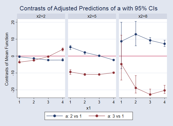
On this case, among the confidence intervals are so slender that they’re exhausting to see. If we glance intently on the blue level on the far left, we see that the arrogance interval for the distinction evaluating a=2 versus a=1 when x1=1 and x2=2 (similar to the primary line within the output above) does embody 0. This means that there’s not a big distinction in these anticipated values. We are able to study every of the opposite factors and confidence intervals in the identical approach. For instance, wanting on the purple line and factors within the third panel, we see that the impact of shifting from a=1 to a=3 is detrimental and considerably totally different from 0 for x1 values of two, 3, and 4. When x1 is 1, the purpose estimate of the impact continues to be detrimental, however that impact just isn’t considerably totally different from 0 on the 95% degree. However recall that we should always dramatically enhance the variety of bootstrap replicates to make any actual claims about confidence intervals.
Up to now, we now have in contrast each a=2 with a=1 and a=3 with a=1. However we aren’t restricted to creating comparisons with a=1. We may evaluate 1 with 2 and a couple of with 3, which frequently makes extra sense if ranges of a have a pure ordering. To do that, we simply exchange r. with ar. in our margins command. I gained’t present that output, however you might have the information and may attempt it should you like.
Inhabitants-averaged outcomes
Up to now, we now have talked about evaluating particular person factors in your response floor and the right way to carry out assessments evaluating anticipated values at these factors. Now, let’s swap gears and speak about population-averaged outcomes.
We’re going to want the dataset to be consultant of the inhabitants. If that’s not true of your knowledge, you’ll want to cease with the analyses we did above. We’ll assume our knowledge are consultant in order that we are able to reply quite a lot of questions primarily based on common predictions.
First, what’s the total anticipated inhabitants imply from this response floor?
. margins, reps(10)
(working margins on estimation pattern)

Bootstrap replications (10)
----+--- 1 ---+--- 2 ---+--- 3 ---+--- 4 ---+--- 5
..........

Predictive margins                              Variety of obs     =      1,497
                                                Replications      =         10

Expression   : imply perform, predict()

------------------------------------------------------------------------------
             |   Noticed   Bootstrap                          Percentile
             |     Margin   Std. Err.      z    P>|z|     [95% Conf. Interval]
-------------+----------------------------------------------------------------
       _cons |   15.64238    .318746    49.07   0.000     15.34973    16.24543
------------------------------------------------------------------------------
Regardless of the course of was that generated this, we imagine 15.6 is the anticipated worth within the inhabitants and [15.3, 16.2] is the arrogance intervals for it.
Do the inhabitants averages differ once we first set everybody to have a=1, then set everybody to have a=2, and at last set everybody to have a=3? Let’s have a look at the anticipated means for all three.
. margins a, reps(10)
(working margins on estimation pattern)

Bootstrap replications (10)
----+--- 1 ---+--- 2 ---+--- 3 ---+--- 4 ---+--- 5
..........

Predictive margins                              Variety of obs     =      1,497
                                                Replications      =         10

Expression   : imply perform, predict()

------------------------------------------------------------------------------
             |   Noticed   Bootstrap                          Percentile
             |     Margin   Std. Err.      z    P>|z|     [95% Conf. Interval]
-------------+----------------------------------------------------------------
           a |
          1  |   18.39275   .4847808    37.94   0.000     17.63322    19.31199
          2  |   19.90499   .6840056    29.10   0.000     18.17305    20.57171
          3  |   8.155515   .3239624    25.17   0.000      7.59187     8.70898
------------------------------------------------------------------------------
We get 18.4, 19.9, and eight.2. They certain don’t look the identical. Let’s check them.
. margins r.a, reps(10)
(working margins on estimation pattern)

Bootstrap replications (10)
----+--- 1 ---+--- 2 ---+--- 3 ---+--- 4 ---+--- 5
..........
Contrasts of predictive margins
                                                Variety of obs     =      1,497
                                                Replications      =         10

Expression   : imply perform, predict()

------------------------------------------------
             |         df        chi2     P>chi2
-------------+----------------------------------
           a |
   (2 vs 1)  |          1       17.10     0.0000
   (3 vs 1)  |          1      618.86     0.0000
      Joint  |          2     1337.66     0.0000
------------------------------------------------

--------------------------------------------------------------
             |   Noticed   Bootstrap          Percentile
             |   Distinction   Std. Err.     [95% Conf. Interval]
-------------+------------------------------------------------
           a |
   (2 vs 1)  |   1.512241   .3656855      1.051265    2.016566
   (3 vs 1)  |  -10.23723   .4115157     -10.82644     -9.4265
--------------------------------------------------------------
Within the causal-inference or treatment-effects literature, the means could be thought-about potential-outcome means, and these variations could be the common remedy results of a multivalued remedy. Right here the common remedy impact of a=2 (in contrast with a=1) is 1.5.
We noticed within the earlier part that variations in anticipated values for ranges of a different throughout values of x2. Let’s estimate the potential-outcome means and remedy results of a at totally different values of x2. Discover that these are nonetheless inhabitants averages as a result of, not like within the earlier part, we aren’t setting x1 to any particular worth. As an alternative, predictions use the noticed values of x1 within the knowledge.
. margins a, at(x2=(2 5 8)) reps(10)
(working margins on estimation pattern)

Bootstrap replications (10)
----+--- 1 ---+--- 2 ---+--- 3 ---+--- 4 ---+--- 5
..........

Predictive margins                              Variety of obs     =      1,497
                                                Replications      =         10

Expression   : imply perform, predict()

1._at        : x2              =           2

2._at        : x2              =           5

3._at        : x2              =           8

------------------------------------------------------------------------------
             |   Noticed   Bootstrap                          Percentile
             |     Margin   Std. Err.      z    P>|z|     [95% Conf. Interval]
-------------+----------------------------------------------------------------
       _at#a |
        1 1  |   3.707771   .6552861     5.66   0.000     4.619393     6.70335
        1 2  |   1.340815   .9491373     1.41   0.158     2.077606    5.010682
        1 3  |   3.677883    .935561     3.93   0.000      4.33317    7.380818
        2 1  |   17.16092     .27028    63.49   0.000      16.8047    17.75164
        2 2  |   17.22508   .1993421    86.41   0.000     16.91111    17.57034
        2 3  |   6.933778   .1929387    35.94   0.000     6.751693    7.332845
        3 1  |   30.61528   .9961323    30.73   0.000     28.66033    31.88367
        3 2  |   40.17685   1.687315    23.81   0.000     36.18359    41.73811
        3 3  |   10.97667   .9771489    11.23   0.000     9.510952    12.59133
------------------------------------------------------------------------------
As an alternative of wanting on the output, let’s graph these potential-outcome means.
. marginsplot
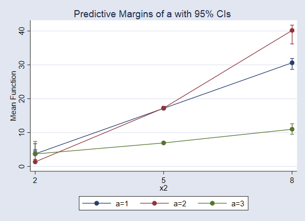
The impact of a will increase as x2 will increase. The impact is largest when x2=8.
Now, we are able to check for variations at every degree of x2
. margins r.a, at(x2=(2 5 8)) reps(10)
(working margins on estimation pattern)

Bootstrap replications (10)
----+--- 1 ---+--- 2 ---+--- 3 ---+--- 4 ---+--- 5
..........
Contrasts of predictive margins
                                                Variety of obs     =      1,497
                                                Replications      =         10

Expression   : imply perform, predict()

1._at        : x2              =           2

2._at        : x2              =           5

3._at        : x2              =           8

------------------------------------------------
             |         df        chi2     P>chi2
-------------+----------------------------------
       a@_at |
 (2 vs 1) 1  |          1       51.80     0.0000
 (2 vs 1) 2  |          1        0.13     0.7184
 (2 vs 1) 3  |          1       43.16     0.0000
 (3 vs 1) 1  |          1        0.01     0.9322
 (3 vs 1) 2  |          1      834.54     0.0000
 (3 vs 1) 3  |          1      245.45     0.0000
      Joint  |          6     2732.16     0.0000
------------------------------------------------

--------------------------------------------------------------
             |   Noticed   Bootstrap          Percentile
             |   Distinction   Std. Err.     [95% Conf. Interval]
-------------+------------------------------------------------
       a@_at |
 (2 vs 1) 1  |  -2.366956   .3288861     -2.737075   -1.466043
 (2 vs 1) 2  |   .0641596   .1779406      -.224935    .3180577
 (2 vs 1) 3  |   9.561575   1.455483      6.847319    11.96769
 (3 vs 1) 1  |  -.0298883   .3513035     -.6345751    .4584875
 (3 vs 1) 2  |  -10.22714   .3540221     -10.89414   -9.808236
 (3 vs 1) 3  |  -19.63861   1.253521     -21.45499    -18.0223
--------------------------------------------------------------
Once more, let’s have a look at the graph.
. marginsplot
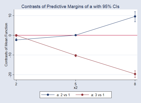
The distinction in means when a=3 and a=1, the remedy impact, just isn’t vital when x2=2. Neither is the impact of a=2 versus a=1 when x2=5. All the opposite results are considerably totally different from 0.
Conclusion
On this weblog, we now have explored the response floor of a nonlinear perform, we now have estimated quite a lot of inhabitants averages primarily based on our nonparametric regression mannequin, and we now have carried out a number of assessments evaluating anticipated values at particular factors of the response floor and assessments evaluating inhabitants averages. But, we now have solely scratched the floor of the kinds of estimates and assessments you may get hold of utilizing margins after npregress. There are extra contrasts operators that may mean you can check variations from a grand imply, variations from technique of earlier or subsequent ranges, and extra. See [R] distinction for particulars of the accessible distinction operators. It’s also possible to use marginsplot to see the outcomes of margins instructions from totally different angles. As an illustration, if we kind marginsplot, bydimension(x1) as a substitute of marginsplot, bydimension(x2), we see our nonlinear response floor from a unique perspective. See [R] marginsplot for particulars and examples of this command.
Whether or not you utilize nonparametric regression or one other mannequin, margins and marginsplot are the answer for exploring the outcomes, making inferences, and understanding relationships among the many variables you’re finding out.