

You studying this tells me you want to be taught extra about Excel. This text continues our Excel collection, the place we explored the VLOOKUP operate within the final iteration. The whole VLOOKUP information demonstrated how the operate works and the way finest to make use of it. This time, we will convey the identical focus to conditional logic and formulation just like the IF operate in Excel. The goal is to know the various kinds of conditional logics and know the best way to use their operators in a working operate inside Excel.
So, no fluff wanted right here. Let’s merely dive in, beginning with what Conditional Logic in Excel is.
What’s Conditional Logic in Excel?
Conditional logic in Excel means making choices primarily based on a situation. In easy phrases, Excel checks a rule you outline, evaluates the end result, after which performs an motion primarily based on that consequence.
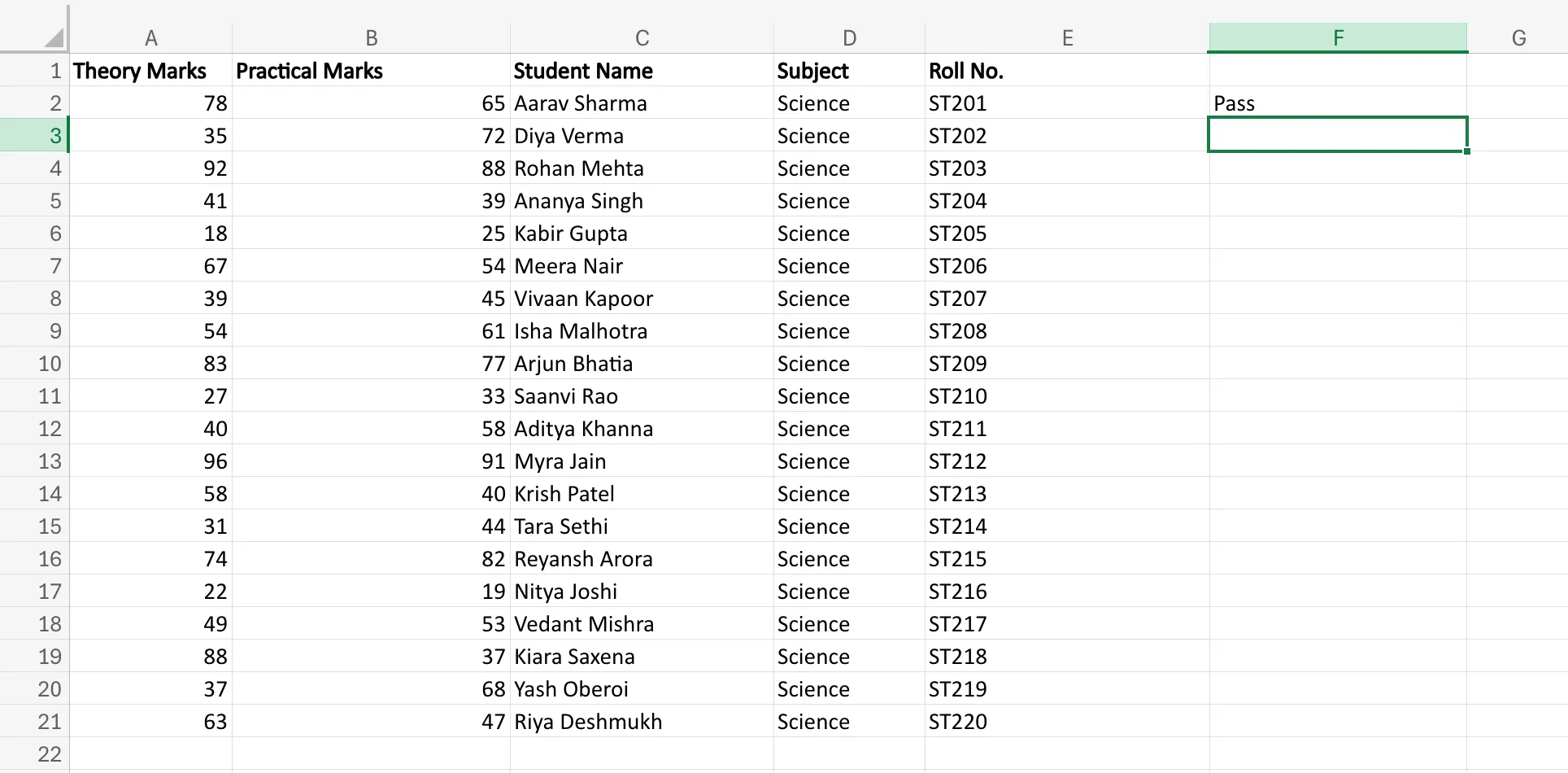
For instance, suppose you’ve got college students’ marks in a sheet and wish to determine whether or not a pupil has handed or failed. Reasonably than checking every worth manually, you may merely apply a situation: if the marks are 40 or above, return “Move”; in any other case, return “Fail”. That’s conditional logic in motion.
The identical logic is used throughout many real-world duties in Excel. You would possibly wish to mark gross sales above a goal as “Achieved”, classify bills as “Excessive” or “Low”, or determine whether or not a fee is “Pending” or “Accomplished”. In every case, Excel is evaluating a situation and returning an output primarily based on the end result.
On the core of this course of is an easy thought:
check a situation > get a TRUE or FALSE end result > use that end result to determine what occurs subsequent.
Such conditional logic is precisely what makes Excel greater than only a spreadsheet for storing knowledge. Its formulation react to values dynamically, reducing down on hours of guide work.
To make this conditional logic work, Excel depends on conditional operators, that are the symbols used to match values. Subsequent, allow us to find out about conditional operators intimately.
Additionally learn: 50+ Excel Interview Inquiries to Ace Your Interview
What are Conditional Operators in Excel?
Give it some thought, how precisely will you evaluate values inside Excel for any conditional logic to work? You will have comparability symbols for various circumstances, like equal (=), higher than (>), smaller than (<), and so on., proper? All such comparability symbols are known as conditional operators in Excel. In essence, these are used to check whether or not a situation is true or false. They’re the constructing blocks behind conditional logic, as a result of they permit Excel to match values earlier than a operate decides what to return.
In easy phrases, these operators assist Excel reply questions like:
- Is that this worth higher than 50?
- Is that this cell equal to “Sure”?
- Are these two values totally different?
- Has the goal been met or not?
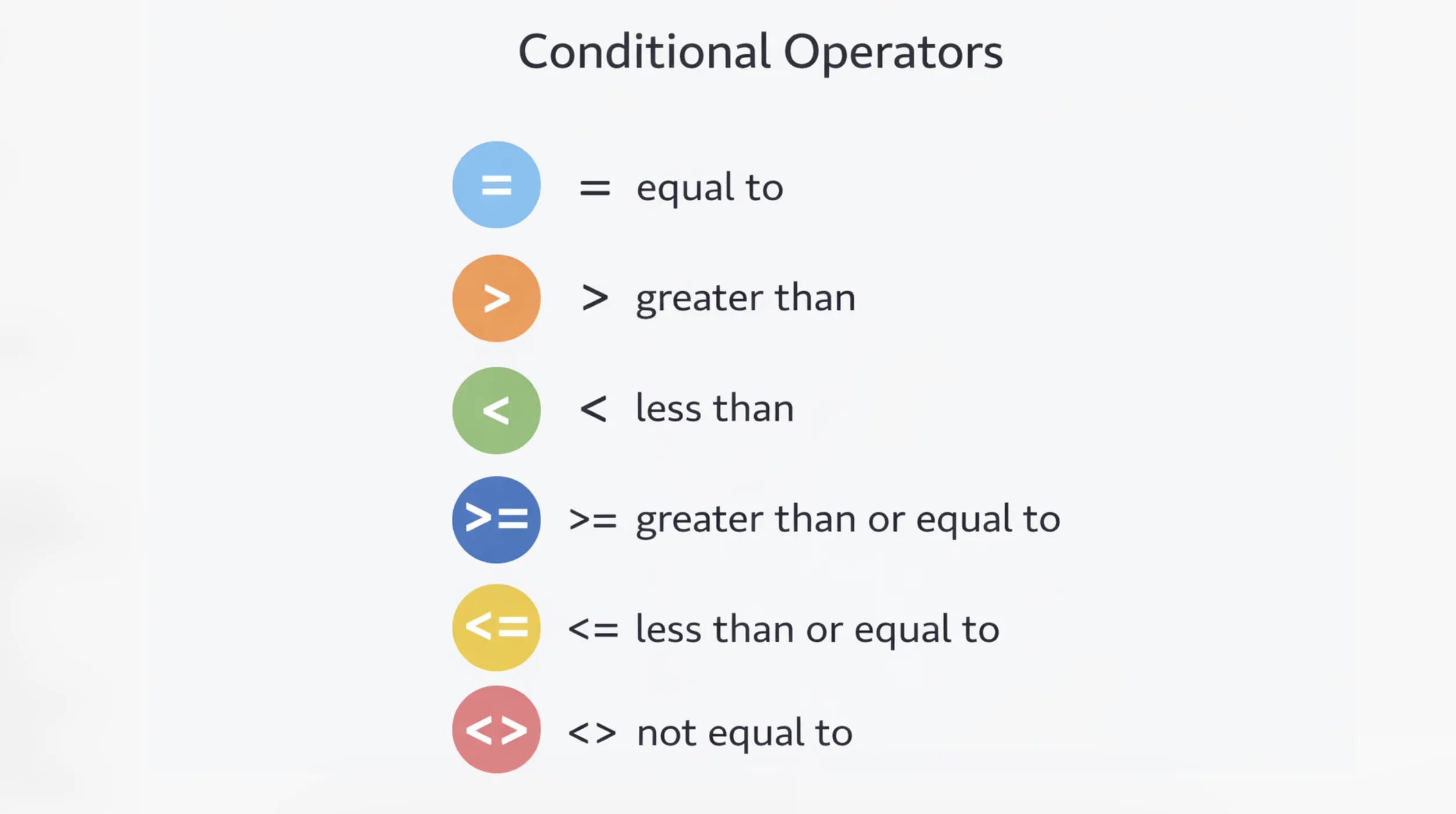
Excel helps six primary conditional operators:
- `=` : equal to
- `>` : higher than
- `<` : lower than
- `>=` : higher than or equal to
- `<=` : lower than or equal to
- `<>` : not equal to
Allow us to perceive this with a easy instance. Suppose cell `A2` comprises the worth `75`.
=A2>50Excel checks whether or not 75 is bigger than 50. Since that situation is true, the components returns `TRUE`.
Now have a look at this:
=A2<50This time, Excel checks whether or not 75 is lower than 50. Since that’s not true, the result’s `FALSE`.
That `TRUE` or `FALSE` output is what powers conditional formulation in Excel. Capabilities like `IF`, `IFS`, `AND`, and `OR` depend on these comparisons to make choices.
For instance:
=IF(A2>=40,"Move","Fail")Don’t fear, we’ll be taught in regards to the IF operate intimately shortly. For now, simply observe on this instance that Excel first checks whether or not the worth in `A2` is bigger than or equal to 40. If the situation is true, it returns `Move`. If the situation is fake, it returns `Fail`. Extra importantly, observe that even the IF operate begins with a conditional operator.
So, whereas capabilities like `IF` usually get all the eye, the actual decision-making begins with these operators. They’re what inform Excel the best way to consider a situation within the first place.
Now that the operators are clear, the following step is to know the conditional capabilities wherein they’re used, beginning with the `IF` operate.
Additionally learn: Microsoft Excel for Knowledge Evaluation
IF Perform in Excel
The IF operate is among the most generally used formulation in Excel. In its most simple sense, it checks whether or not a situation is true or false, after which returns a end result primarily based on that consequence. In easy phrases, it tells Excel: if this occurs, do that; in any other case, try this.
To know it correctly, allow us to break it into two elements.
IF Perform Syntax
The syntax of the IF operate is:
=IF(logical_test, value_if_true, value_if_false)Right here, every half has a selected position:
- logical_test is the situation Excel checks
- value_if_true is the end result returned if the situation is true
- value_if_false is the end result returned if the situation is fake
Allow us to have a look at a easy instance:
=IF(A2>=40,"Move","Fail")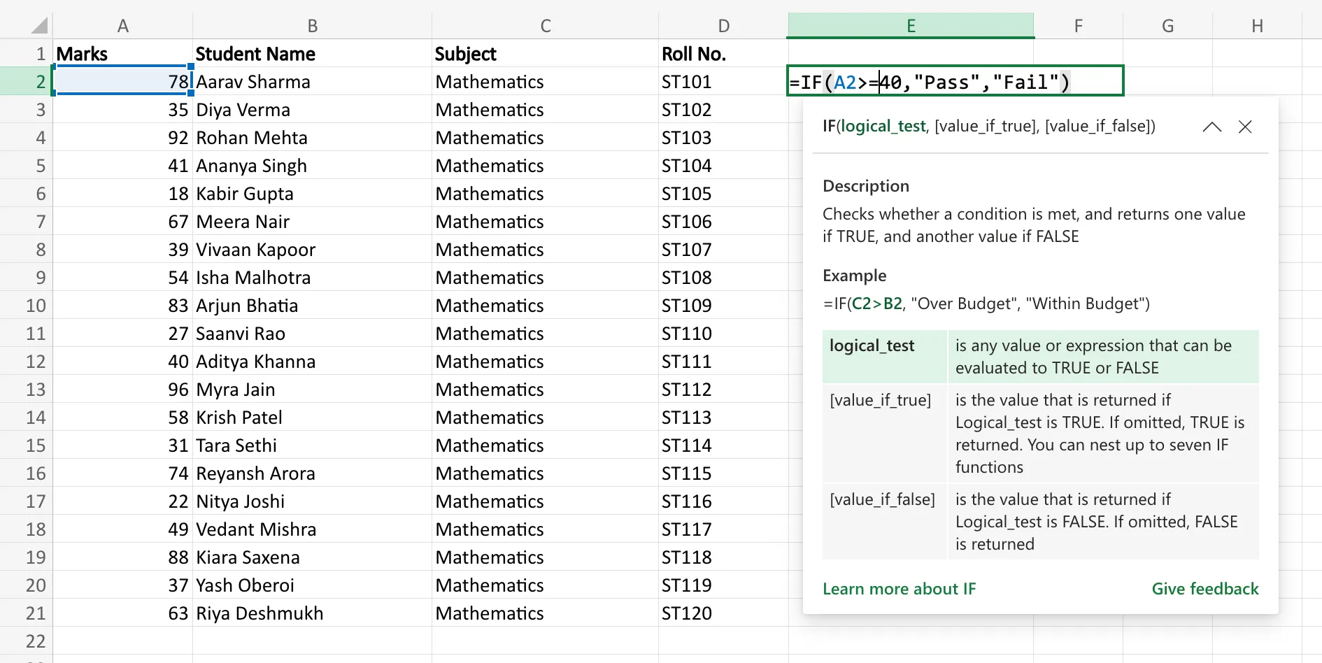
Here’s what Excel is doing on this components:
- It first checks whether or not the worth in cell A2 is bigger than or equal to 40
- If that situation is true, Excel returns Move
- If that situation is fake, Excel returns Fail
So, if A2 comprises 65, the end result will probably be Move. If it comprises 28, the end result will probably be Fail.
That is the essential construction of each IF components. First, Excel evaluates the situation. Then it decides which end result to return.
Forming the Method
Now that the syntax is obvious, the following step is to really construct the components in Excel.
Suppose you’ve got marks listed in column A, and also you wish to present the lead to column B.
Begin by clicking the cell the place you need the output to look. Then kind:
=IF(A2>=40,"Move","Fail")Press Enter, and Excel will immediately return the end result primarily based on the worth in A2.
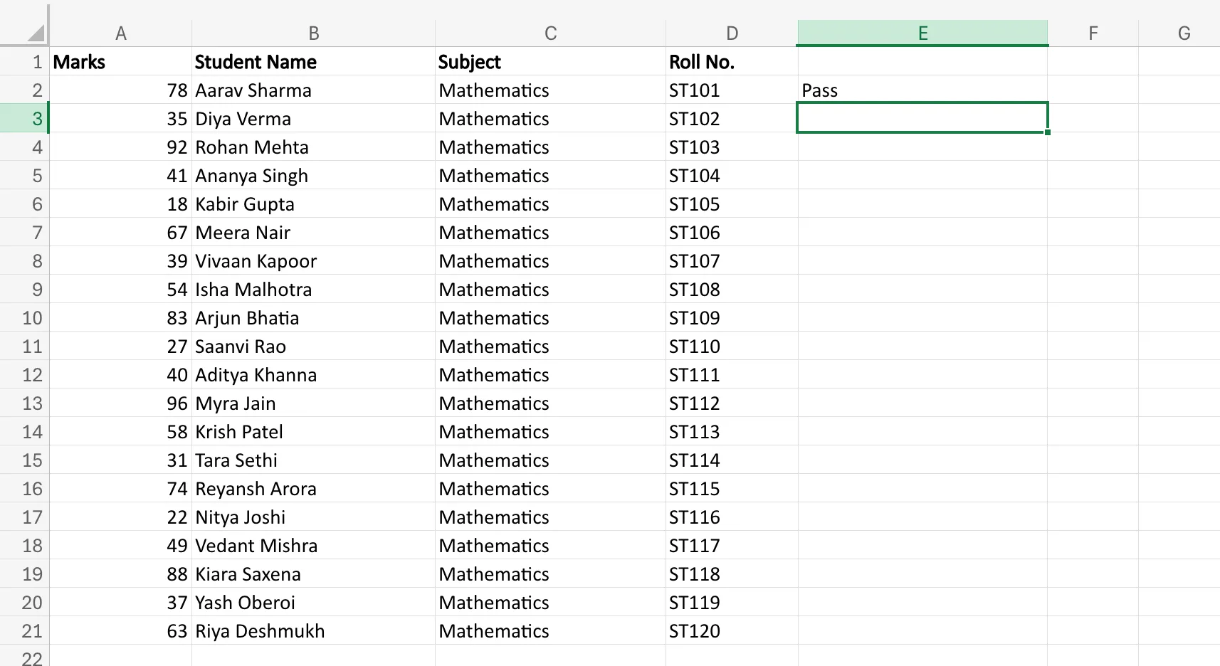
For the reason that worth meets the situation on this case, you get ‘Move’. If it didn’t, you’ll get ‘Fail’.
As soon as the components works in a single cell, you may drag it down to use the identical logic to the remainder of the rows. Excel will routinely modify the cell reference for every row.
As an example:
- in row 2, Excel checks A2
- in row 3, it checks A3
- in row 4, it checks A4
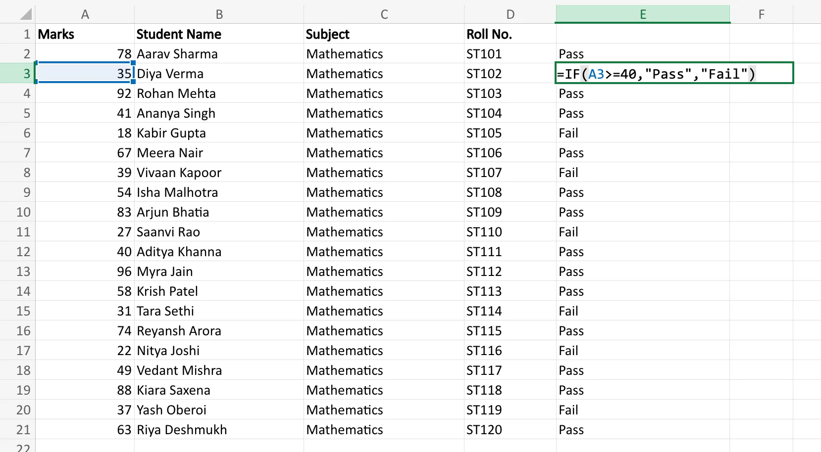
That is what makes the IF operate so helpful. You create the logic as soon as, and Excel repeats it throughout the dataset in seconds.
Now that we perceive how a single IF components works, the following step is to see what occurs when there are greater than two potential outcomes. That’s the place Nested IF statements are available in.
Nested IF Statements in Excel
A single `IF` operate works nicely when there are solely two outcomes. However many actual Excel duties contain greater than only a yes-or-no choice. You could have to assign grades, label efficiency bands, or categorise values into a number of teams. That’s the place Nested IF statements are available in.
A Nested IF merely means putting one `IF` operate inside one other, so Excel can check a number of circumstances one after the opposite.
Nested IF Syntax
Contemplate a easy Excel sheet that has the marks of scholars saved as knowledge, and you must grade the scholars primarily based on their marks. A primary Nested IF components for a similar will look one thing like this:
=IF(A2>=90,"A",IF(A2>=75,"B",IF(A2>=40,"C","Fail")))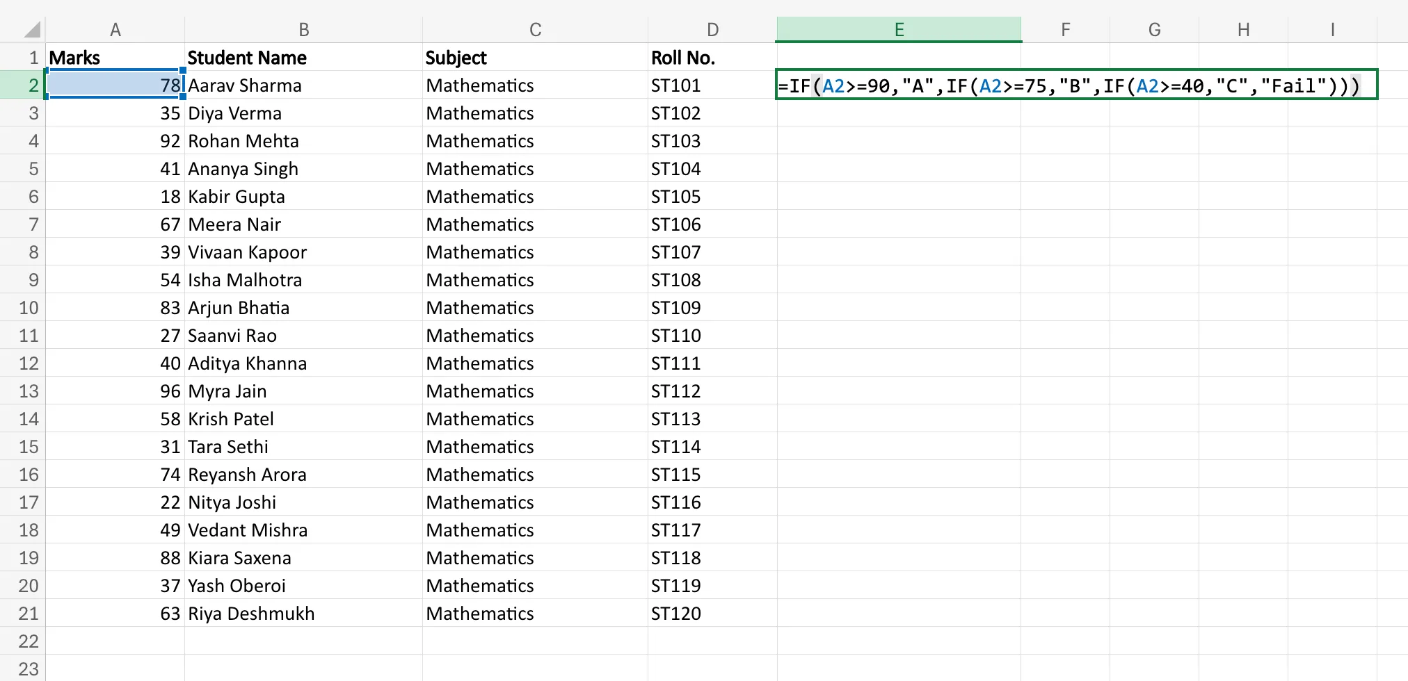
This will look intimidating at first, however the logic is easy. Excel checks every situation in sequence:
- If `A2` is 90 or above, it returns `A`
- If not, it checks whether or not `A2` is 75 or above, and returns `B`
- If not, it checks whether or not `A2` is 40 or above, and returns `C`
- If none of those circumstances are met, it returns `Fail`
So if `A2` comprises 82, the components returns `B`. If it comprises 36, Excel returns `Fail`.
The important thing factor to know right here is that Excel stops as quickly because it finds the primary true situation. It doesn’t maintain checking the remainder.
Forming the Method
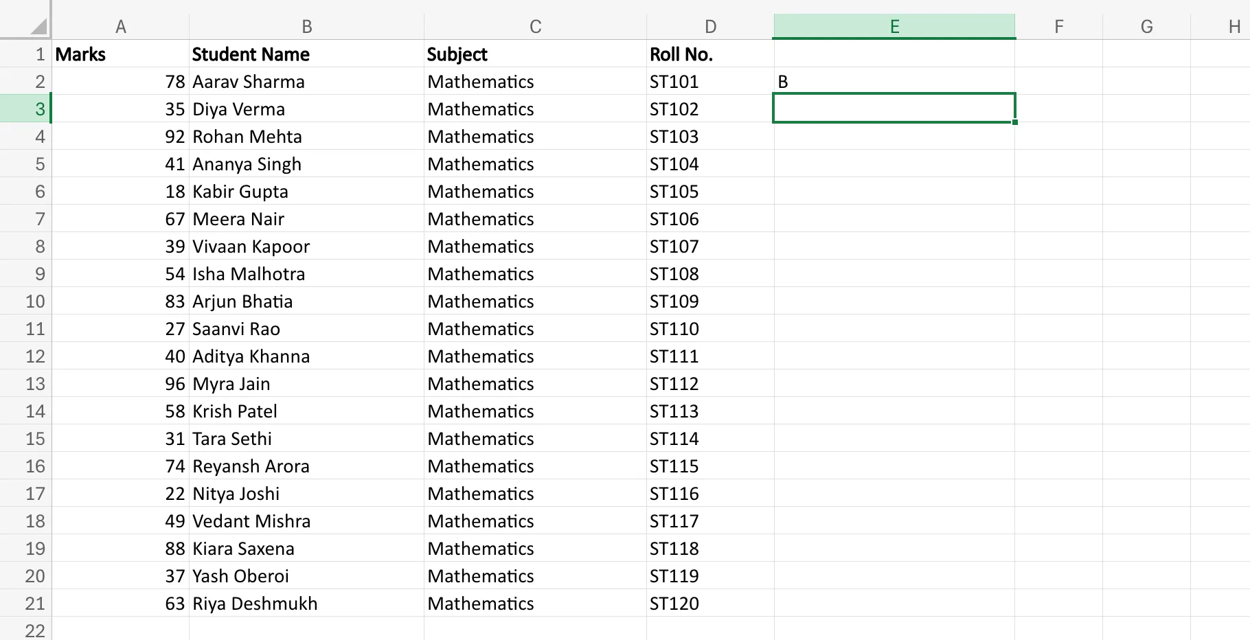
Suppose you’ve got pupil marks in column `A`, and also you wish to assign grades in column `B`.
Click on the output cell and enter:
=IF(A2>=90,"A",IF(A2>=75,"B",IF(A2>=40,"C","Fail")))Then press Enter.
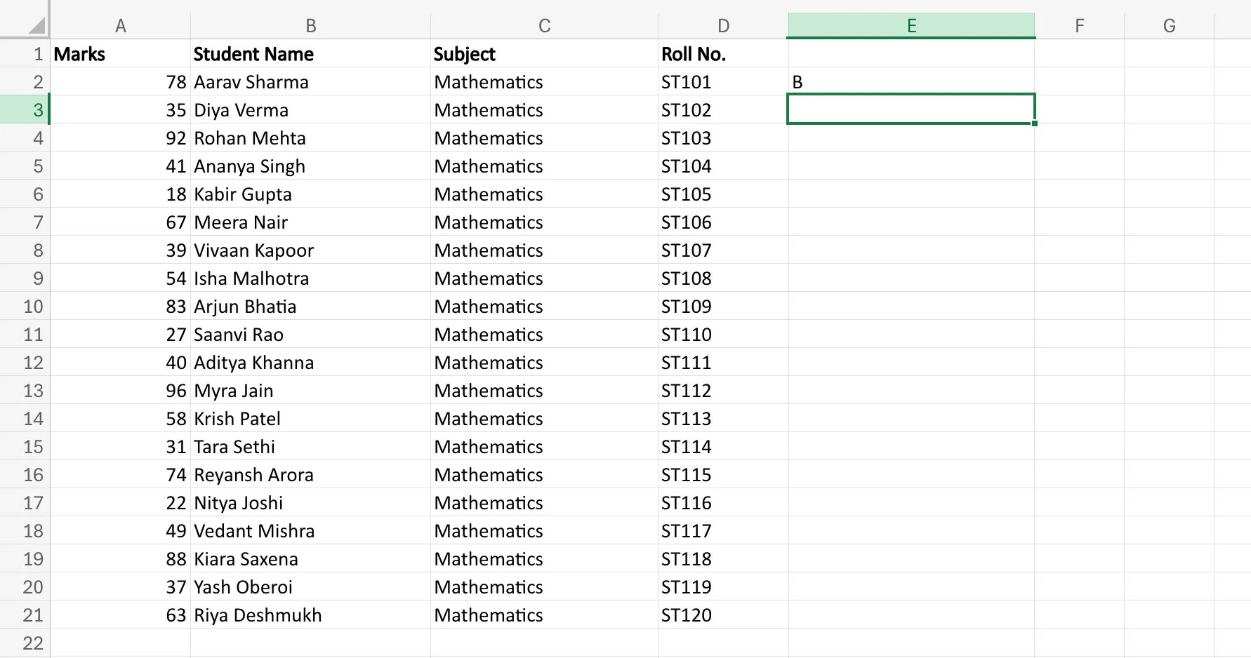
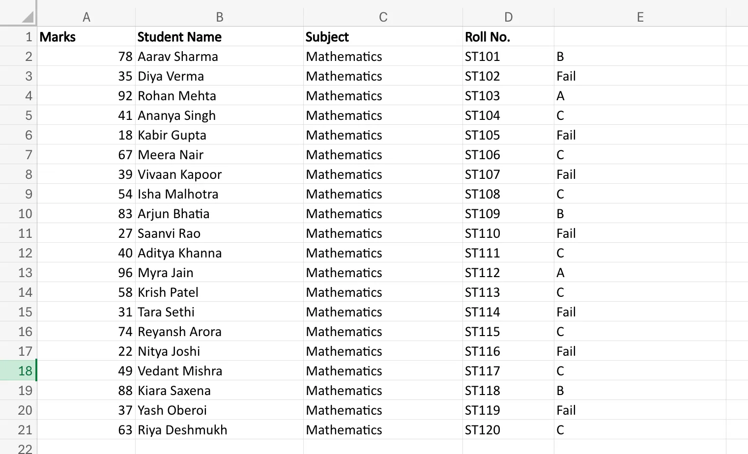
Excel will consider the circumstances from left to proper and return the right grade for that row. As soon as the components works, drag it down to use the identical grading logic to the remainder of the info, as seen within the picture beneath.
One necessary factor to recollect: the order of circumstances issues. Within the instance above, the best rating vary is checked first. Should you reverse the order carelessly, Excel could return the improper end result.
Nested IF statements are helpful, however they will change into tough to learn when too many circumstances are concerned. That’s precisely why Excel launched a cleaner different known as `IFS`.
Additionally learn: 10 Most Generally Used Statistical Capabilities in Excel
IFS Perform in Excel
Think about if, within the grading instance above, you had grades as much as Z at hand out. The Nested `IF` statements could get the job achieved, however will certainly change into very messy, in a short time. When you begin stacking a number of circumstances inside each other, the components turns into tougher to learn, tougher to edit, and simpler to interrupt. That’s the place the `IFS` operate helps.
The `IFS` operate is designed to check a number of circumstances in a cleaner format. As a substitute of nesting one `IF` inside one other, you record every situation and its lead to sequence.
IFS Perform Syntax
The syntax of the `IFS` operate is:
=IFS(logical_test1, value_if_true1, logical_test2, value_if_true2, ...)Every logical check is adopted by the end result Excel ought to return when that situation is true.
Allow us to take the identical grading instance we utilized in Nested IF:
=IFS(A2>=90,"A",A2>=75,"B",A2>=40,"C",A2<40,"Fail")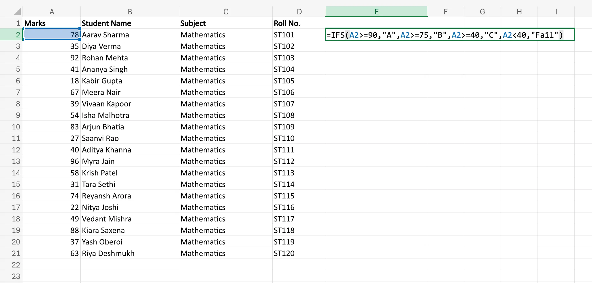
Here’s what Excel does:
- If `A2` is 90 or above, it returns `A`
- If not, it checks whether or not `A2` is 75 or above, and returns `B`
- If not, it checks whether or not `A2` is 40 or above, and returns `C`
- If `A2` is beneath 40, it returns `Fail`
The logic is much like Nested IF, however the construction is far cleaner. You wouldn’t have to maintain observe of a number of closing brackets inside brackets.
Forming the Method
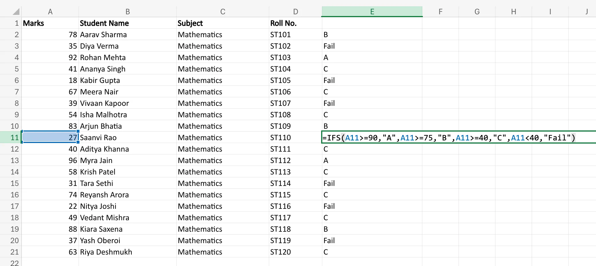
Suppose marks are listed in column `A`, and also you need grades in column `B`.
Click on the output cell and kind:
=IFS(A2>=90,"A",A2>=75,"B",A2>=40,"C",A2<40,"Fail")Then press Enter.
Excel will check the circumstances so as and return the end result for the primary situation that evaluates to true. After that, you may drag the components down for the remainder of the rows.
This makes `IFS` particularly helpful when you’ve got a number of potential outcomes and wish the components to remain readable.
That stated, `IFS` is finest if you end up checking a number of separate circumstances. However typically the problem will not be a number of outcomes. Typically you wish to check multiple situation on the identical time. For that, Excel makes use of `AND` and `OR` capabilities.
AND and OR Capabilities in Excel
Up to now, we have now checked out formulation the place Excel checks one situation at a time. However in actual spreadsheets, a single situation is commonly not sufficient. It’s your decision a end result solely when a number of circumstances are true, or when at the least one out of a number of circumstances is true. That is the place `AND` and `OR` are available in.
Each are logical capabilities in Excel, and they’re normally used inside formulation like `IF`.
AND Perform Syntax
The `AND` operate returns `TRUE` solely when all circumstances are true.
Its syntax is:
=AND(logical1, logical2, ...)Allow us to say a pupil passes provided that they rating greater than 40 in idea and greater than 40 in sensible.
=AND(A2>40,B2>40)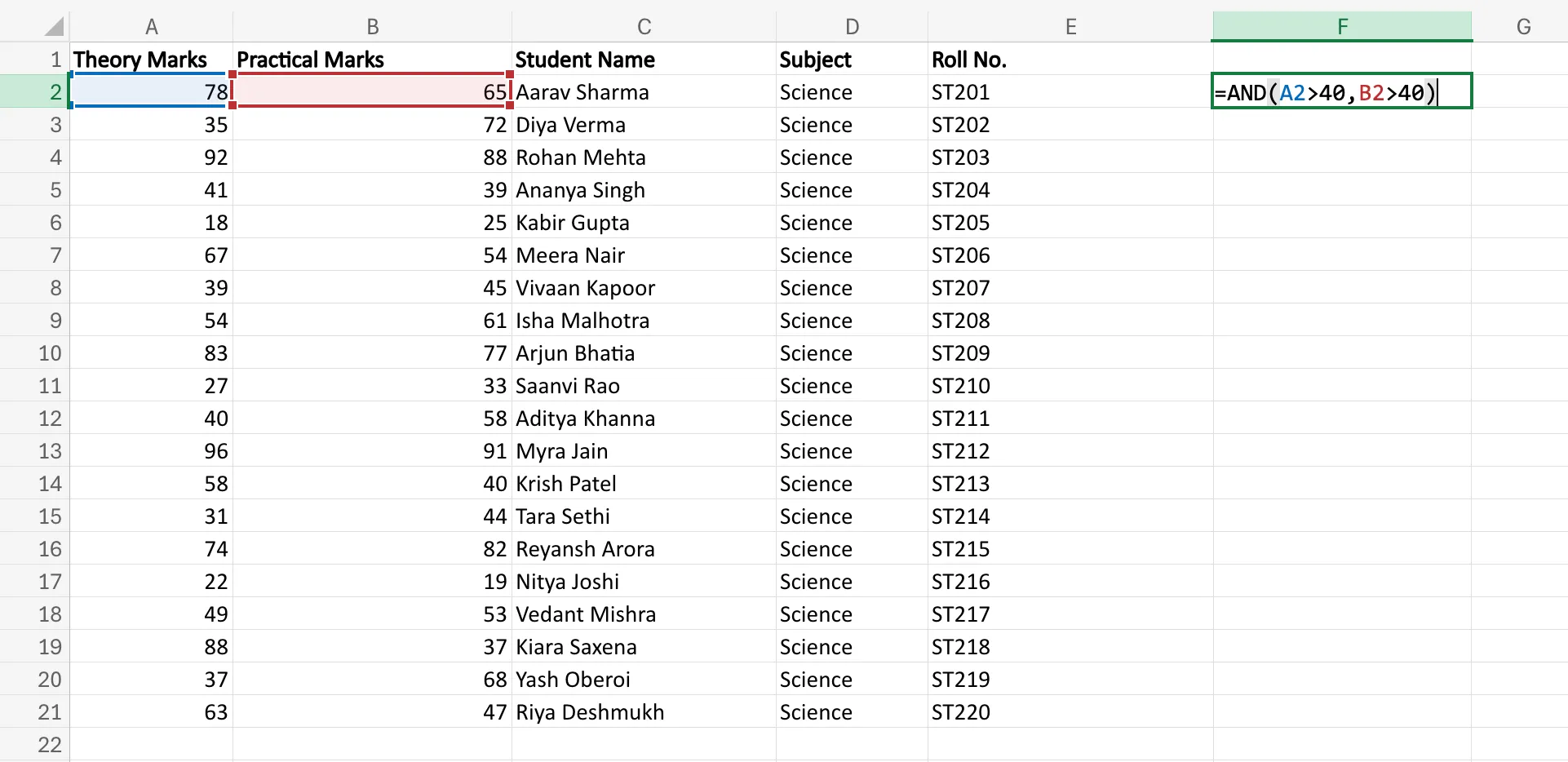
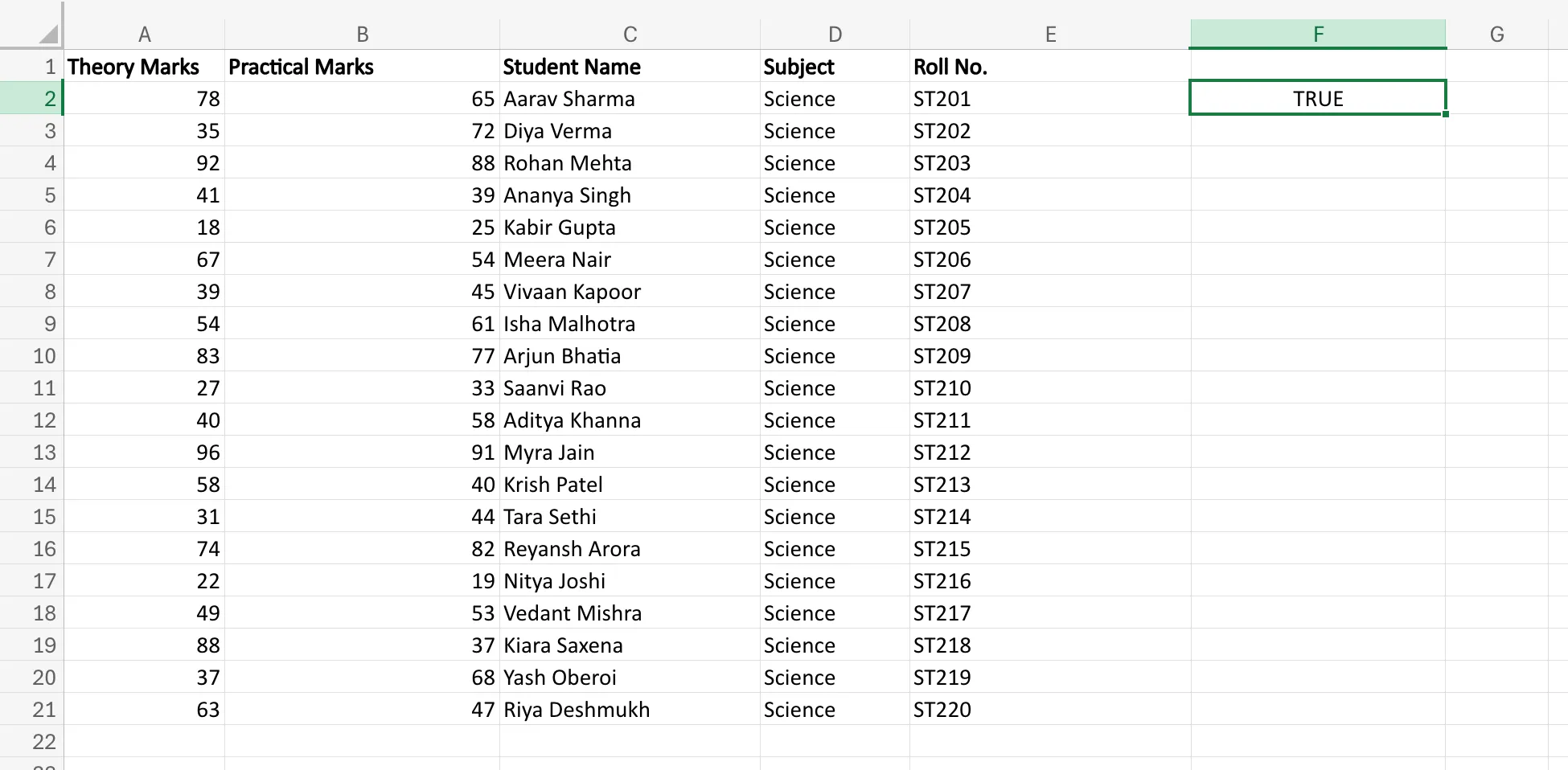
Right here, Excel checks each circumstances:
- Is `A2` higher than 40?
- Is `B2` higher than 40?
If each are true, Excel returns `TRUE`. If even one is fake, Excel returns `FALSE`.
Now allow us to use it inside an `IF` operate:
=IF(AND(A2>40,B2>40),"Move","Fail")
This tells Excel to return Move provided that each circumstances are happy. In any other case, it returns Fail.
OR Perform Syntax
The `OR` operate works in a different way. It returns `TRUE` when at the least one situation is true.
Its syntax is:
=OR(logical1, logical2, ...)Suppose a salesman qualifies for a bonus in the event that they both cross a gross sales goal or usher in a brand new consumer.
=OR(A2>=100000,B2="Sure")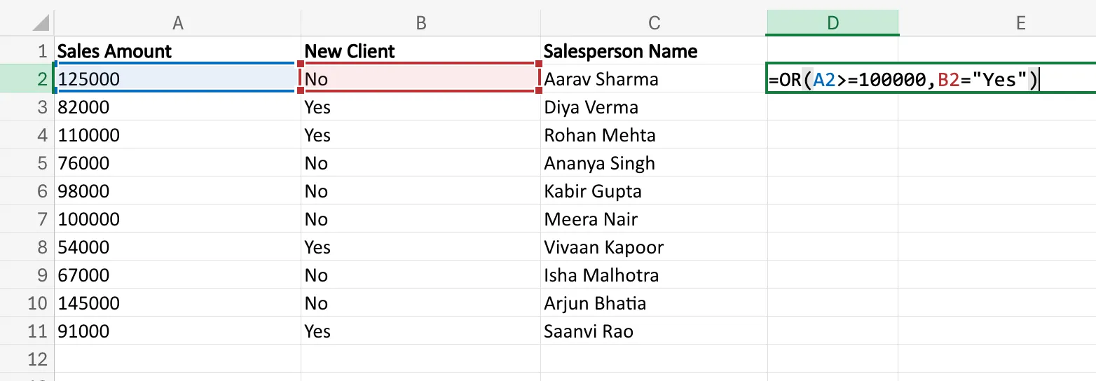
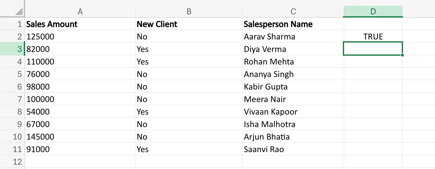
Right here, Excel checks:
- Is `A2` higher than or equal to 100000?
- Is `B2` equal to “Sure”?
If even one in all these is true, Excel returns `TRUE`.
Used inside `IF`, it turns into:
=IF(OR(A2>=100000,B2="Sure"),"Bonus Eligible","Not Eligible")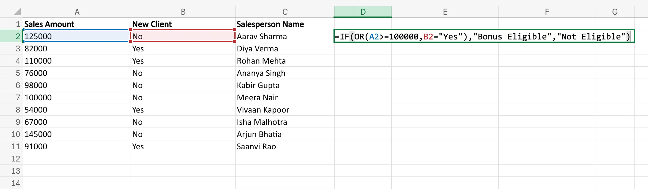
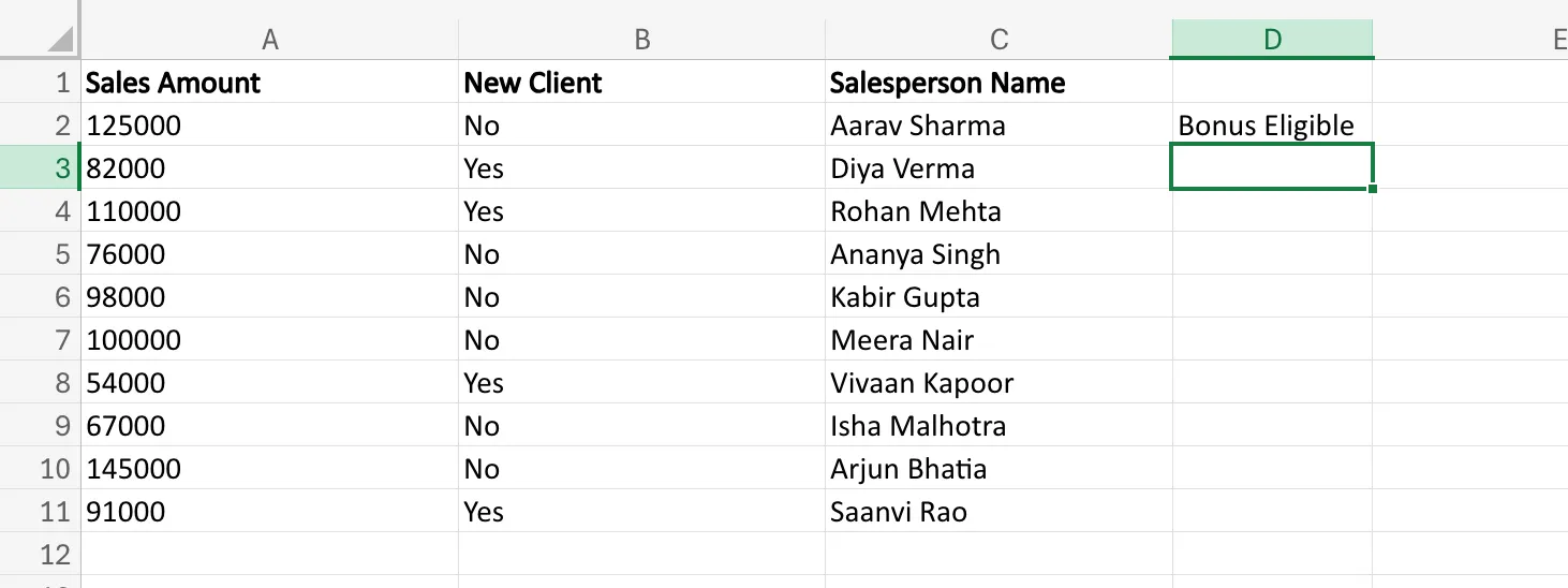
So if the particular person meets both one of many circumstances, Excel marks them as Bonus Eligible.
Forming the Method
The simplest option to construct these formulation is to first determine your logic clearly.
- Use `AND` when each situation have to be met.
- Use `OR` when only one situation is sufficient.
For instance, if an worker will get approval solely once they have accomplished coaching and submitted paperwork, you’ll write:
=IF(AND(A2="Sure",B2="Sure"),"Permitted","Pending")But when they will qualify by way of both of two routes, you’ll use:
=IF(OR(A2="Sure",B2="Sure"),"Permitted","Pending")That’s the core distinction. `AND` is stricter. `OR` is extra versatile.
These capabilities change into particularly highly effective when mixed with `IF`, as a result of they permit Excel to deal with extra practical decision-making guidelines. However even then, formulation can nonetheless break if the info throws an error. That’s the place `IFERROR` and `IFNA` change into helpful.
IFERROR and IFNA in Excel
Even when your logic is right, Excel formulation don’t at all times return clear outcomes. Typically they produce errors as a result of a price is lacking, a lookup fails, or the components can not course of the enter. That’s the place `IFERROR` and `IFNA` change into helpful.
These capabilities show you how to exchange ugly error messages with one thing extra significant and readable. As a substitute of exhibiting `#VALUE!`, `#DIV/0!`, or `#N/A`, you may ask Excel to return a customized output.
IFERROR Perform Syntax
The `IFERROR` operate checks whether or not a components returns any error. If it does, Excel reveals the worth you specify as an alternative.
Its syntax is:
=IFERROR(worth, value_if_error)Right here:
- `worth` is the components or expression Excel ought to consider
- `value_if_error` is what Excel ought to return if the components leads to an error
Allow us to have a look at an instance:
=IFERROR(A2/B2,"Error in Calculation")Right here, Excel tries to divide `A2` by `B2`.
- If the division works, Excel returns the precise end result
- If the components throws an error, corresponding to division by zero, Excel returns Error in Calculation
That is helpful as a result of it retains your worksheet cleaner and simpler to know.
Forming the IFERROR Method
Suppose you’re calculating proportion progress, and there’s a probability that the earlier worth is zero. A traditional division components could return an error. To keep away from that, you may wrap the components inside `IFERROR`:
=IFERROR((B2-A2)/A2,"Not Obtainable")Press Enter, and Excel will both present the expansion worth or return **Not Obtainable** if the components breaks.
This helps lots in stories and dashboards, the place error values could make the sheet look messy or complicated.
IFNA Perform Syntax
The `IFNA` operate is extra particular. It solely handles the `#N/A` error, which normally seems when a lookup components can not discover a match.
Its syntax is:
=IFNA(worth, value_if_na)Allow us to take a easy instance with `VLOOKUP`:
=IFNA(VLOOKUP(E2,A2:C10,2,FALSE),"Not Discovered")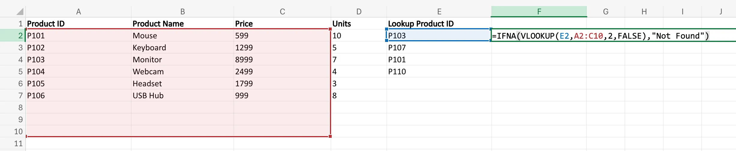
Right here, Excel tries to seek out the worth from `E2` contained in the vary `A2:C10`.
- If a match is discovered, it returns the corresponding end result
- If no match is discovered and Excel produces `#N/A`, it returns Not Discovered
That is higher than exhibiting `#N/A` to the reader, particularly in lookup-based sheets.
Forming the IFNA Method
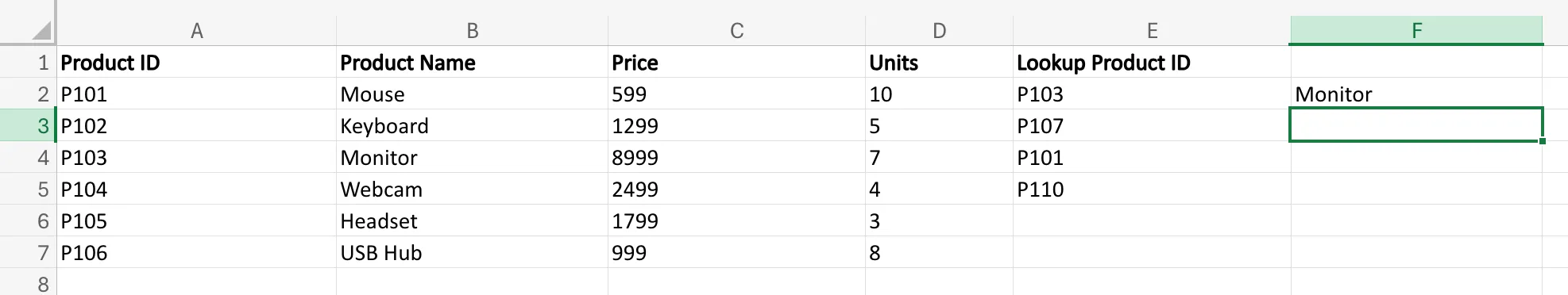
Suppose you’ve got a product ID in cell `E2`, and also you wish to fetch the product identify from a lookup desk. If the ID doesn’t exist, you don’t want Excel to indicate an error.
So as an alternative of writing solely:
=VLOOKUP(E2,A2:C10,2,FALSE)you may write:
=IFNA(VLOOKUP(E2,A2:C10,2,FALSE),"Product Not Discovered")This makes the output way more user-friendly.
IFERROR vs IFNA
The distinction is straightforward:
- `IFERROR` handles all forms of errors
- `IFNA` handles solely the `#N/A` error
So if you’re coping with lookups and solely wish to catch lacking matches, `IFNA` is extra exact. However if you’d like a broader security web for any error, `IFERROR` is the higher alternative.
At this level, we have now coated the important thing Excel capabilities that energy conditional logic: `IF`, Nested `IF`, `IFS`, `AND`, `OR`, `IFERROR`, and `IFNA`. The ultimate step is to convey every part along with a sensible conclusion on when to make use of every one.
Additionally learn: Superior Excel for Knowledge Evaluation
Conclusion
As you begin utilizing these formulation in your Excel sheets extra usually, you’ll realise the period of time every of those can prevent. These capabilities are what make Excel really feel like a working choice system. As a substitute of simply storing numbers and textual content, Excel can consider circumstances, apply guidelines, and return the suitable solutions routinely. Therefore, these formulation like `IF`, `IFS`, `AND`, `OR`, `IFERROR`, and `IFNA` have a lot sensible worth.
To sum up, the `IF` operate is the start line whenever you want Excel to decide on between two outcomes. Nested `IF` helps when these outcomes improve. `IFS` presents a cleaner option to deal with a number of circumstances with out turning the components right into a bracket jungle. `AND` and `OR` take the logic additional by permitting you to check a number of circumstances collectively, relying on whether or not all or simply one in all them must be true. Lastly, `IFERROR` and `IFNA` assist make your spreadsheets extra readable by changing error messages with helpful outputs.
Since they’ve such excessive sensible worth, the actual good thing about studying these capabilities is the power to make spreadsheets smarter, cleaner, and way more helpful in actual work. When you perceive how conditional logic works, you realise the ability of Excel relating to decoding knowledge.
Login to proceed studying and luxuriate in expert-curated content material.