

Introduction
Dynamic stochastic normal equilibrium (DSGE) fashions are utilized in macroeconomics to mannequin the joint conduct of mixture time sequence like inflation, rates of interest, and unemployment. They’re used to research coverage, for instance, to reply the query, “What’s the impact of a shock rise in rates of interest on inflation and output?” To reply that query we’d like a mannequin of the connection amongst rates of interest, inflation, and output. DSGE fashions are distinguished from different fashions of a number of time sequence by their shut connection to financial concept. Macroeconomic theories encompass programs of equations which can be derived from fashions of the selections of households, corporations, policymakers, and different brokers. These equations type the DSGE mannequin. As a result of the DSGE mannequin is derived from concept, its parameters may be interpreted immediately when it comes to the idea.
On this put up, I construct a small DSGE mannequin that’s just like fashions used for financial coverage evaluation. I present learn how to estimate the parameters of this mannequin utilizing the brand new dsge command in Stata 15. I then shock the mannequin with a contraction in financial coverage and graph the response of mannequin variables to the shock.
A small DSGE mannequin
A DSGE mannequin begins with an outline of the sectors of the financial system to be modeled. The mannequin I describe right here is said to the fashions developed in Clarida, Galí, and Gertler (1999) and Woodford (2003). It’s a smaller model of the sorts of fashions utilized in central banks and academia for financial coverage evaluation. The mannequin has three sectors: households, corporations, and a central financial institution.
- Households devour output. Their choice making is summarized by an output demand equation that relates present output demand to anticipated future output demand and the actual rate of interest.
- Companies set costs and produce output to fulfill demand on the set value. Their choice making is summarized by a pricing equation that relates present inflation (that’s, the change in costs) to anticipated future inflation and present demand. The parameter capturing the diploma to which inflation is dependent upon output demand performs a key function within the mannequin.
- The central financial institution units the nominal rate of interest in response to inflation. The central financial institution will increase the rate of interest when inflation rises and reduces the rate of interest when inflation falls.
The mannequin may be summarized in three equations,
start{align}
x_t &= E_t(x_{t+1}) – {r_t – E_t(pi_{t+1}) – z_t}
pi_t &= beta E_t(pi_{t+1}) + kappa x_t
r_t &= frac{1}{beta} pi_t + u_t
finish{align}
The variable (x_t) denotes the output hole. The output hole measures the distinction between output and its future, pure worth. The notation (E_t(x_{t+1})) specifies the expectation, conditional on data obtainable at time (t), of the output hole in interval (t+1). The nominal rate of interest is (r_t), and the inflation fee is (pi_t). Equation (1) states that the output hole is said positively to the anticipated future output hole, (E_t(x_{t+1})), and negatively to the rate of interest hole, ({r_t – E_t(pi_{t+1}) – z_t}). The second equation is the agency’s pricing equation; it relates inflation to anticipated future inflation and the output hole. The parameter (kappa) determines the extent to which inflation is dependent upon the output hole. Lastly, the third equation summarizes the central financial institution’s conduct; it relates the rate of interest to inflation and to different elements, collectively termed (u_t).
The endogenous variables (x_t), (pi_t), and (r_t) are pushed by two exogenous variables, (z_t) and (u_t). By way of the idea, (z_t) is the pure fee of curiosity. If the actual rate of interest is the same as the pure fee and is predicted to stay so sooner or later, then the output hole is zero. The exogenous variable (u_t) captures all actions within the rate of interest that come up from elements apart from actions in inflation. It’s generally known as the shock part of financial coverage.
The 2 exogenous variables are modeled as first-order autoregressive processes,
start{align}
z_{t+1} &= rho_z z_t + varepsilon_{t+1}
u_{t+1} &= rho_u u_t + xi_{t+1}
finish{align}
which follows frequent observe.
Within the jargon, endogenous variables are known as management variables, and exogenous variables are known as state variables. The values of management variables in a interval are decided by the system of equations. Management variables may be noticed or unobserved. State variables are mounted at first of a interval and are unobserved. The system of equations determines the worth of state variables one interval sooner or later.
We want to use the mannequin to reply coverage questions. What’s the impact on mannequin variables when the central financial institution conducts a shock enhance within the rate of interest? The reply to this query is to impose an impulse (xi_t) and hint out the impact of the impulse over time.
Earlier than doing coverage evaluation, we should assign values to the parameters of the mannequin. We are going to estimate the parameters of the above mannequin utilizing U.S. information on inflation and rates of interest with dsge in Stata.
Specifying the DSGE to dsge
I match the mannequin utilizing information on the U.S. rate of interest and inflation fee. In a DSGE mannequin, you’ll be able to have as many observable management variables as you might have shocks within the mannequin. As a result of the mannequin has two shocks, we now have two observable management variables. The variables in a linearized DSGE mannequin are stationary and measured in deviation from regular state. In observe, this implies the information should be de-meaned previous to estimation. dsge will take away the imply for you.
I take advantage of the information in usmacro2, which is drawn from the Federal Reserve Financial institution of St. Louis database.
. webuse usmacro2
To specify a mannequin to Stata, sort the equations utilizing substitutable expressions.
. dsge (x = E(F.x) - (r - E(F.p) - z), unobserved) ///
       (p = {beta}*E(F.p) + {kappa}*x)             ///
       (r = 1/{beta}*p + u)                        ///
       (F.z = {rhoz}*z, state)                     ///
       (F.u = {rhou}*u, state)
The foundations for equations are just like these for Stata’s different instructions that work with substitutable expressions. Every equation is certain in parentheses. Parameters are enclosed in braces to tell apart them from variables. Expectations of future variables seem throughout the E() operator. One variable seems on the left-hand facet of the equation. Additional, every variable within the mannequin seems on the left-hand facet of 1 and just one equation. Variables may be both noticed (exist as variables in your dataset) or unobserved. As a result of the state variables are mounted within the present interval, equations for state variables categorical how the one-step-ahead worth of the state variable is dependent upon present state variables and, presumably, present management variables.
Estimating the mannequin parameters offers us an output desk:
. dsge (x = E(F.x) - (r - E(F.p) - z), unobserved) ///
>      (p = {beta}*E(F.p) + {kappa}*x)             ///
>      (r = 1/{beta}*p + u)                        ///
>      (F.z = {rhoz}*z, state)                     ///
>      (F.u = {rhou}*u, state)
(setting method to bfgs)
Iteration 0:   log probability = -13738.863
Iteration 1:   log probability = -1311.9615  (backed up)
Iteration 2:   log probability = -1024.7903  (backed up)
Iteration 3:   log probability = -869.19312  (backed up)
Iteration 4:   log probability = -841.79194  (backed up)
(switching method to nr)
Iteration 5:   log probability =  -819.0268  (not concave)
Iteration 6:   log probability =  -782.4525  (not concave)
Iteration 7:   log probability = -764.07067
Iteration 8:   log probability = -757.85496
Iteration 9:   log probability = -754.02921
Iteration 10:  log probability = -753.58072
Iteration 11:  log probability = -753.57136
Iteration 12:  log probability = -753.57131

DSGE mannequin

Pattern: 1955q1 - 2015q4                         Variety of obs     =        244
Log probability = -753.57131
------------------------------------------------------------------------------
             |                 OIM
             |      Coef.   Std. Err.      z    P>|z|     [95% Conf. Interval]
-------------+----------------------------------------------------------------
/structural  |
        beta |    .514668    .078349     6.57   0.000     .3611067    .6682292
       kappa |   .1659046    .047407     3.50   0.000     .0729885    .2588207
        rhoz |   .9545256   .0186424    51.20   0.000     .9179872     .991064
        rhou |   .7005492   .0452603    15.48   0.000     .6118406    .7892578
-------------+----------------------------------------------------------------
      sd(e.z)|   .6211208   .1015081                      .4221685     .820073
      sd(e.u)|     2.3182   .3047433                      1.720914    2.915486
------------------------------------------------------------------------------
The essential parameter is {kappa}, which is estimated to be optimistic. This parameter is said to the underlying value frictions within the mannequin. Its interpretation is that if we maintain anticipated future inflation fixed, a 1 share level enhance within the output hole results in a 0.17 share level enhance in inflation.
The parameter (beta) is estimated to be about 0.5, which means that the coefficient on inflation within the rate of interest equation is about 2. So the central financial institution will increase the rate of interest about two for one in response to actions in inflation. This parameter is way mentioned within the financial economics literature, and estimates of it cluster round 1.5. The worth discovered right here is comparable with these estimates. Each state variables (z_t) and (u_t) are estimated to be persistent, with autoregressive coefficients of 0.95 and 0.7, respectively.
Impulse–responses
We are able to now use the mannequin to reply questions. One query the mannequin can reply is, “What’s the impact of an surprising change within the rate of interest on inflation and the output hole?” An surprising change within the rate of interest is modeled as a shock to the (u_t) equation. Within the language of the mannequin, this shock represents a contraction in financial coverage.
An impulse is a sequence of values for the shock (xi) in (5): ((1, 0, 0, 0, 0, dots)). The shock then feeds into the mannequin’s state variables, resulting in a rise in (u). From there, the rise in (u) results in a change in all of the mannequin’s management variables. An impulse–response perform traces out the impact of a shock on the mannequin variables, taking into consideration all of the interrelationships amongst variables current within the mannequin equations.
We sort three instructions to construct and graph an IRF. irf set units the IRF file that can maintain the impulse–responses. irf create creates a set of impulse–responses within the IRF file.
. irf set dsge_irf
. irf create model1
With the impulse–responses saved, we are able to graph them:
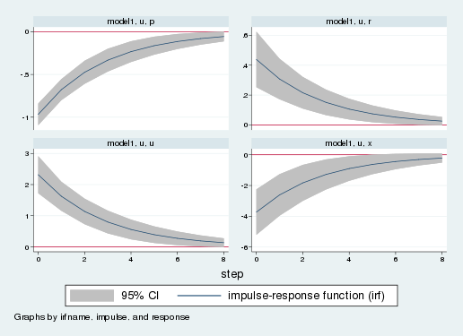
. irf graph irf, impulse(u) response(x p r u) byopts(yrescale) yline(0)
The impulse–response graphs the response of mannequin variables to a one-standard-deviation shock. Every panel is the response of 1 variable to the shock. The horizontal axis measures time for the reason that shock, and the vertical axis measures deviations from long-run worth. The underside-left panel exhibits the response of the financial state variable, (u_t). The remaining three panels present the response of inflation, the rate of interest, and the output hole. Inflation is within the top-left panel; it falls on affect of the shock. The rate of interest response within the upper-right panel is a weighted sum of the inflation and financial impulse–responses. The rate of interest rises by about one-half of 1 share level. Lastly, the output hole falls. Therefore, the mannequin predicts that after a financial tightening, the financial system will enter a recession. Over time, the impact of the shock dissipates, and all variables return to their long-run values.
Conclusion
On this put up, I developed a small DSGE mannequin and described learn how to estimate the parameters of the mannequin utilizing dsge. I then confirmed learn how to create and interpret an impulse–response perform.
References
Clarida, R., J. Galí, and M. Gertler. 1999. The science of financial coverage: A brand new Keynesian perspective. Journal of Financial Literature 37: 1661–1707.
Woodford, M. 2003. Curiosity and Costs: Foundations of a Idea of Financial Coverage. Princeton, NJ: Princeton College Press.