

I’ve a confession. I wasn’t excited concerning the addition of frames to Stata 16. Sure, frames has been probably the most requested options for a few years, and our web site analytics present that frames is wildly fashionable. Including frames was a good move and our clients are excited. However I’ve used Stata for over 20 years, and I’ve been completely joyful utilizing one dataset at a time. So I ignored frames.
Then I began engaged on an instance for lasso utilizing genetic information. I simulated affected person information together with genetic information for every of twenty-two chromosomes saved in 22 separate datasets. Working with 23 datasets grew to become cumbersome, so I assumed I’d take a look at frames. I started by studying the handbook after which tinkered with my genetic information. Alongside the best way, I found a function of frames that fully blew my thoughts. I’m going to indicate you that function under, and I anticipate that it’ll blow your thoughts as nicely.
This weblog publish shouldn’t be meant to be an introduction to frames. There’s a detailed introduction to frames within the Stata 16 handbook that may make you an professional. I merely need to present you among the helpful issues that you are able to do with frames, together with the next:
- Use a number of datasets concurrently
- Frames and postestimation
- Linked frames and frval()
- Linked frames and frget
- Many frames
Use a number of datasets concurrently
On this instance, I’ve simulated affected person information in a single dataset and information from the NHANES research, which is a nationally consultant pattern of individuals in the USA. I want to evaluate the outcomes of regression fashions utilizing my information with the outcomes utilizing the NHANES information. The NHANES information comprise survey weights and my information don’t. It may be potential to append the 2 datasets right into a single dataset and use an indicator variable to distinguish between the observations from every research. However it will be troublesome and irritating to suit fashions with survey weights for some observations and never others. That is simple utilizing frames.
Let’s start by utilizing body create to create a brand new information body named sufferers. Then, we are able to use the body prefix to make use of the affected person information within the information body sufferers.
. body create sufferers

. body sufferers: use sufferers
We are able to then create one other information body named nhanes2 and webuse the dataset nhanes2.
. body create nhanes2

. body nhanes2: webuse nhanes2
We are able to sort body dir to confirm that we have now three information frames in reminiscence. One is known as default and the opposite two are the frames we created. We are able to additionally see the variety of observations, the variety of variables, and the datasets which might be contained in every body.
. body dir
  default   0 x 0
  nhanes2   10351 x 58; nhanes2.dta
  sufferers  10000 x 41; sufferers.dta
Now, we are able to use the frames prefix to suit a linear regression mannequin with out survey weights utilizing the affected person information. And we are able to use the frames prefix to suit the identical regression mannequin with survey weights utilizing the NHANES information. Be aware that I’ve used estimates retailer to retailer the parameter estimates in reminiscence.
body sufferers: regress sbp c.age##c.bmi
(output omitted)
estimates retailer sufferers
body nhanes2: svy linearized : regress bpsystol c.age##c.bmi
(output omitted)
estimates retailer nhanes
Now, we are able to evaluate the outcomes of our mannequin match to the 2 datasets utilizing estimates desk.
. estimates desk sufferers nhanes

----------------------------------------
    Variable |  sufferers      nhanes
-------------+--------------------------
         age |   .5587357    .51511664
         bmi |   1.259132    1.2066527
             |
 c.age#c.bmi |  .00742543    .00200162
             |
       _cons |  70.882924     72.51606
----------------------------------------
Frames and postestimation
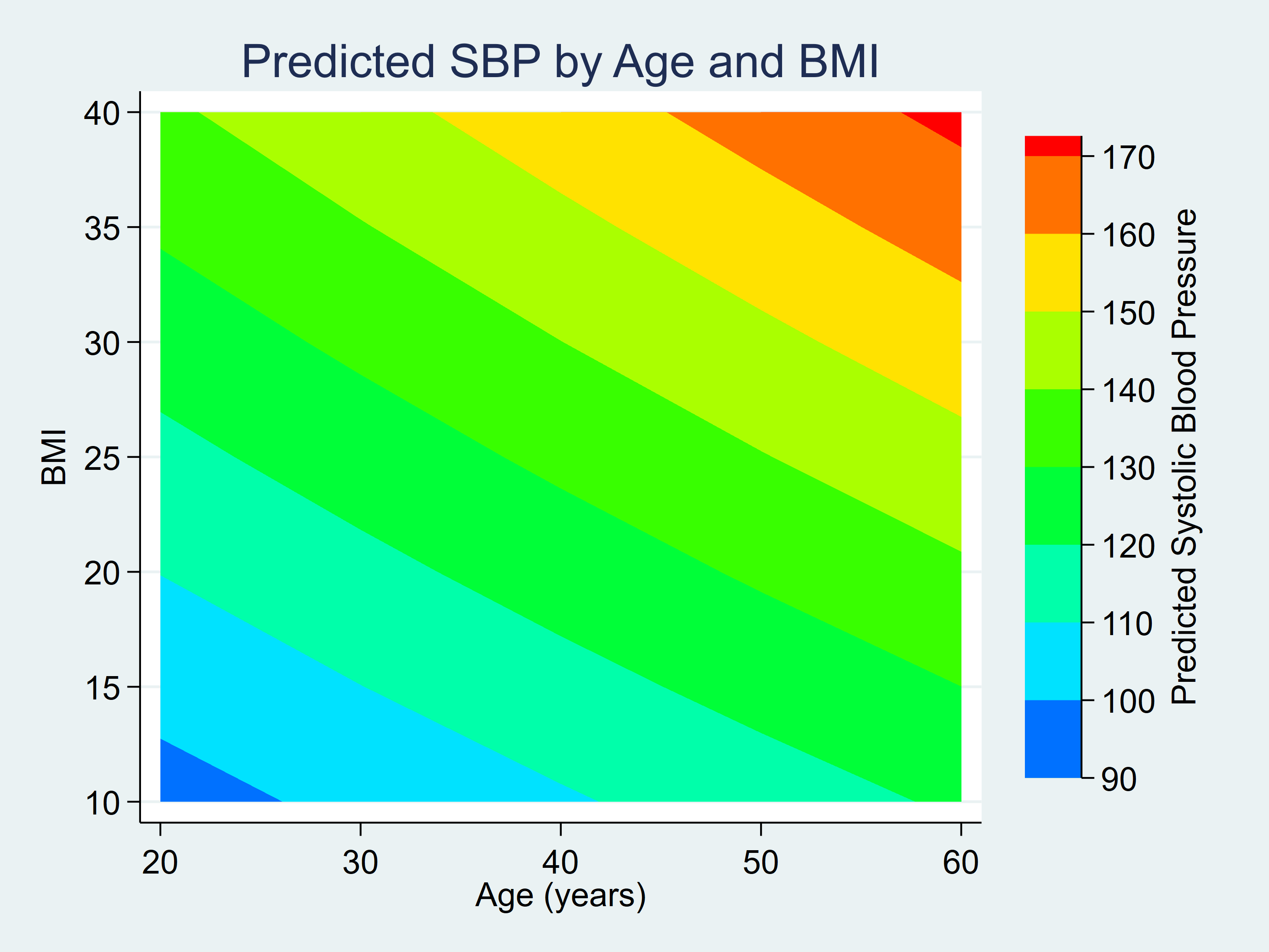
Subsequent, we’d want to graph the predictions from the mannequin utilizing our affected person information. We are able to do that utilizing a method that I describe in a Stata Information article titled Visualizing continuous-by-continuous interactions with margins and twoway contour.
The fundamental technique is to suit the mannequin, use margins to estimate and save the predictions to a dataset, then use graph twoway contour to create the graph. Within the Stata Information article, I needed to clear the primary dataset to open the predictions dataset. Right here we are able to merely create one other body to make use of the dataset that accommodates our predictions.
Let’s start by utilizing body change in order that we are able to run a number of instructions utilizing the affected person information. Then we are able to match our regression mannequin and estimate the predictions utilizing margins. Be aware that I’ve included the choice saving(predictions, exchange), which tells margins to retailer the predictions to a dataset named predictions.
. body change sufferers

. regress sbp c.age##c.bmi

      Supply |       SS           df       MS      Variety of obs   =    10,000
-------------+----------------------------------   F(3, 9996)      =  14015.35
       Mannequin |   1670892.7         3  556964.234   Prob > F        =    0.0000
    Residual |  397237.042     9,996  39.7396001   R-squared       =    0.8079
-------------+----------------------------------   Adj R-squared   =    0.8079
       Whole |  2068129.74     9,999  206.833658   Root MSE        =    6.3039

------------------------------------------------------------------------------
         sbp |      Coef.   Std. Err.      t    P>|t|     [95% Conf. Interval]
-------------+----------------------------------------------------------------
         age |   .5587357   .0865853     6.45   0.000     .3890112    .7284602
         bmi |   1.259132   .1758975     7.16   0.000     .9143375    1.603927
             |
 c.age#c.bmi |   .0074254   .0034766     2.14   0.033     .0006105    .0142404
             |
       _cons |   70.88292   4.305602    16.46   0.000     62.44308    79.32277
------------------------------------------------------------------------------

. margins, at(age=(20(10)60) bmi=(10(5)40)) saving(predictions, exchange)
(Output omitted)
Now, we are able to create a brand new body named contour, change to that body, and use the dataset predictions.
. body create contour

. body change contour

. use predictions
(Created by command margins; additionally see char record)
The variable _at1 within the predictions dataset accommodates age, _at2 accommodates BMI, and _margin accommodates the linear predictions.
. describe _at1 _at2 _margin

              storage   show    worth
variable title   sort    format     label      variable label
------------------------------------------------------------------------
_at1            byte    %9.0g                 age in years
_at2            byte    %9.0f                 Physique Mass Index (BMI)
_margin         float   %9.0g                 Linear prediction, predict()

. record _at1 _at2 _margin in 1/5

     +------------------------+
     | _at1   _at2    _margin |
     |------------------------|
  1. |   20     10   96.13405 |
  2. |   20     15   103.1722 |
  3. |   20     20   110.2104 |
  4. |   20     25   117.2487 |
  5. |   20     30   124.2869 |
     +------------------------+
We are able to rename these variables and create a contour plot of the predictions.
. rename _at1 age

. rename _at2 bmi

. rename _margin pr_sbp

. twoway (contour pr_sbp bmi age, ccuts(90(10)170)),            ///
>         xlabel(20(10)60)  ylabel(10(5)40, angle(horizontal))  ///
>         xtitle("Age (years)") ytitle("BMI")                   ///
>         ztitle("Predicted Systolic Blood Stress")           ///
>         title("Predicted SBP by Age and BMI")
Determine 1: Contour Plot for Predicted SBP by Age and BMI
Linked frames and frval()
We are able to additionally hyperlink two frames collectively utilizing frlink. Let’s open one other dataset named hospital in a brand new body named hospital.
. body create hospital

. body change hospital

. use hospital

. record in 1/5, abbrev(10)

     +----------------------+
     | hospitalid   avgcost |
     |----------------------|
  1. |          1   135,242 |
  2. |          2   135,372 |
  3. |          3   134,467 |
  4. |          4   132,953 |
  5. |          5   134,622 |
     +----------------------+
The hospital dataset accommodates the variable hospitalid and a variable named avgcost, which is the common value of coronary heart bypass surgical procedure at every hospital.
The sufferers dataset accommodates a variable named fee, which is the quantity that every affected person paid for coronary heart bypass surgical procedure. The variable hospitalid tells us the hospital at which every affected person had surgical procedure.
. body change sufferers

. record patientid hospitalid fee in 1/5, abbrev(10)

     +----------------------------------+
     | patientid   hospitalid   fee |
     |----------------------------------|
  1. |         1           10   121,255 |
  2. |         2           18    90,164 |
  3. |         3            5   156,731 |
  4. |         4            6    98,256 |
  5. |         5           13   140,604 |
     +----------------------------------+
We are able to hyperlink the affected person body with the hospital body utilizing frlink. Every worth of hospitalid seems many instances within the sufferers body and solely as soon as within the hospital body. We are able to specify a “many-to-one” hyperlink by typing frlink m:1. And body(hospital) tells frlink to hyperlink the present body (sufferers) with the hospital body.
. frlink m:1 hospitalid, body(hospital)
  (all observations in body sufferers matched)
Now that our frames are linked, we are able to use frval() to entry values of variables in frames outdoors the present body. For instance, we’d want to calculate how a lot a affected person paid for coronary heart bypass surgical procedure relative to the common value on the hospital the place the surgical procedure was carried out. We are able to generate a brand new variable named rel_payment, which is the same as the ratio of fee within the present body (sufferers), divided by avgcost within the hospital body. The operate frval(hospital, avgcost) accesses the worth of avgcost within the hospital body.
. generate rel_payment = fee / frval(hospital, avgcost)

. record patientid hospitalid fee rel_payment in 1/5, abbrev(16)

     +------------------------------------------------+
     | patientid   hospitalid   fee   rel_payment |
     |------------------------------------------------|
  1. |         1           10   121,255      .8999608 |
  2. |         2           18    90,164      .6621906 |
  3. |         3            5   156,731      1.164228 |
  4. |         4            6    98,256      .7454461 |
  5. |         5           13   140,604      1.033123 |
     +------------------------------------------------+
Affected person 3 within the record above paid $156,731 for surgical procedure at Hospital 5. The hospital information above present that the common value of the surgical procedure at Hospital 5 was $134,622. The worth of rel_payment tells us that affected person 3 paid 16% extra for his or her surgical procedure than the common value at hospital 5.
Linked frames and frget
We are able to additionally copy variables from one linked body to a different body utilizing frget. On this instance, we have now one other dataset named longitudinal, which accommodates repeated observations of bmi and sbp over 5 years. Let’s create a brand new information body named lengthy for this dataset.
. body create lengthy

. body change lengthy

. use longitudinal

. record in 1/10, abbrev(10)

     +-----------------------------+
     | patientid   age   bmi   sbp |
     |-----------------------------|
  1. |         1    44    25   139 |
  2. |         1    45    26   144 |
  3. |         1    46    27   147 |
  4. |         1    47    25   137 |
  5. |         1    48    25   139 |
     |-----------------------------|
  6. |         2    69    26   164 |
  7. |         2    70    25   166 |
  8. |         2    71    28   169 |
  9. |         2    72    27   171 |
 10. |         2    73    24   165 |
     +-----------------------------+
We want to match a multilevel mannequin for these longitudinal information saved within the lengthy body, adjusting for the consequences of intercourse and race, that are saved within the sufferers body. Let’s start by utilizing frlink to hyperlink the 2 frames.
. frlink m:1 patientid, body(sufferers)
  (all observations in body lengthy matched)
Subsequent, we are able to use frget to repeat the variables intercourse and race from the sufferers body to the present body (lengthy).
. frget intercourse race, from(sufferers)
  (2 variables copied from linked body)

. record in 1/10, abbrev(10)

     +---------------------------------------------------------+
     | patientid   age   bmi   sbp   sufferers      intercourse    race |
     |---------------------------------------------------------|
  1. |         1    44    25   139          1     Male   White |
  2. |         1    45    26   144          1     Male   White |
  3. |         1    46    27   147          1     Male   White |
  4. |         1    47    25   137          1     Male   White |
  5. |         1    48    25   139          1     Male   White |
     |---------------------------------------------------------|
  6. |         2    69    26   164          2   Feminine   White |
  7. |         2    70    25   166          2   Feminine   White |
  8. |         2    71    28   169          2   Feminine   White |
  9. |         2    72    27   171          2   Feminine   White |
 10. |         2    73    24   165          2   Feminine   White |
     +---------------------------------------------------------+
Now, we are able to match our multilevel mannequin.
. blended sbp i.intercourse i.race c.age##c.bmi || patientid:, nolog noheader

------------------------------------------------------------------------------
         sbp |      Coef.   Std. Err.      z    P>|z|     [95% Conf. Interval]
-------------+----------------------------------------------------------------
         intercourse |
     Feminine  |   .1787433   .1213193     1.47   0.141    -.0590382    .4165247
             |
        race |
      Black  |   .0270491   .1957962     0.14   0.890    -.3567045    .4108026
      Different  |   .0539184   .4375286     0.12   0.902    -.8036219    .9114587
             |
         age |     .48519   .0158596    30.59   0.000     .4541058    .5162742
         bmi |   1.175005   .0322024    36.49   0.000     1.111889     1.23812
             |
 c.age#c.bmi |    .010324   .0006217    16.61   0.000     .0091055    .0115424
             |
       _cons |    72.9325   .8130494    89.70   0.000     71.33895    74.52605
------------------------------------------------------------------------------

------------------------------------------------------------------------------
  Random-effects Parameters  |   Estimate   Std. Err.     [95% Conf. Interval]
-----------------------------+------------------------------------------------
patientid: Id          |
                  var(_cons) |    35.8953   .5189054      34.89254    36.92689
-----------------------------+------------------------------------------------
               var(Residual) |   3.973389   .0280961      3.918702     4.02884
------------------------------------------------------------------------------
LR take a look at vs. linear mannequin: chibar2(01) = 76974.75      Prob >= chibar2 = 0.0000
Many frames
I discussed earlier that I’ve been experimenting with simulated genetic information and lasso. Let’s assume that I despatched blood samples from 500 sufferers to a lab they usually despatched us 22 datasets. Every of the 22 datasets accommodates indicator variables for the presence of a selected genetic marker. Let’s check out the recordsdata.
. ls

  79.6M   7/22/19  9:40  chromosome1.dta
  42.8M   7/22/19  9:40  chromosome10.dta
  43.2M   7/22/19  9:40  chromosome11.dta
  42.6M   7/22/19  9:40  chromosome12.dta
  36.6M   7/22/19  9:40  chromosome13.dta
  34.2M   7/22/19  9:40  chromosome14.dta
  32.6M   7/22/19  9:40  chromosome15.dta
  28.8M   7/22/19  9:40  chromosome16.dta
  26.6M   7/22/19  9:40  chromosome17.dta
  25.7M   7/22/19  9:40  chromosome18.dta
  18.7M   7/22/19  9:40  chromosome19.dta
  77.4M   7/22/19  9:40  chromosome2.dta
  20.6M   7/22/19  9:40  chromosome20.dta
  14.9M   7/22/19  9:40  chromosome21.dta
  16.2M   7/22/19  9:40  chromosome22.dta
  63.4M   7/22/19  9:40  chromosome3.dta
  60.8M   7/22/19  9:40  chromosome4.dta
  58.0M   7/22/19  9:40  chromosome5.dta
  54.6M   7/22/19  9:40  chromosome6.dta
  51.0M   7/22/19  9:40  chromosome7.dta
  46.4M   7/22/19  9:40  chromosome8.dta
  44.3M   7/22/19  9:41  chromosome9.dta
The very first thing that I discover is that every file is pretty massive. The file chromosome1.dta is 79.6 megabytes. Let’s describe the contents of the file chromosome1.dta with out opening the file.
. describe utilizing chromosome1, quick

Comprises information
  obs:           500                          15 Jul 2019 17:30
 vars:        73,090
Sorted by:
This dataset accommodates 500 observations on 73,090 variables, which tells me that I might want to use Stata/MP to open this file. Stata/MP can open recordsdata with as much as 120,000 variables and over 20 billion observations. All of the examples under require Stata/MP.
We may also want to vary a few of Stata’s defaults to work with these massive datasets.
. set segmentsize 100m    // Default is 32m

. set maxvar 80000       // Default is 5000
set segmentsize allocates reminiscence for information in models of segmentsize. Smaller values of segmentsize may end up in extra environment friendly use of obtainable reminiscence however require Stata to leap round extra. Our largest file is chromosome1.dta, which is 79.6 megabytes, so I’ve modified the segmentsize to 100 megabytes.
set maxvar modifications the utmost variety of variables allowed from the default of 5,000 to 80,000.
You possibly can learn extra concerning the particulars of reminiscence administration within the handbook.
Now we’re able to open the dataset chromosome1.dta.
. body create chr1

. body change chr1

. use chromosome1

. record id gene1_snp1 gene1_snp2 gene1_snp3 gene1_snp4 gene1_snp5 in 1/5, abbrev(12)

     +---------------------------------------------------------------------+
     | id   gene1_snp1   gene1_snp2   gene1_snp3   gene1_snp4   gene1_snp5 |
     |---------------------------------------------------------------------|
  1. |  1            0            0            0            1            0 |
  2. |  2            0            0            0            0            0 |
  3. |  3            0            0            0            0            0 |
  4. |  4            1            0            0            1            1 |
  5. |  5            0            0            0            1            0 |
     +---------------------------------------------------------------------+
The record above contains solely 6 of the 73,090 variables within the dataset. The variable id within the lengthy body corresponds to the variable patientid within the sufferers body. So we might want to rename the variable patientid to id earlier than we are able to hyperlink the 2 frames.
. body sufferers: rename patientid id

. frlink 1:1 id, body(sufferers)
  (all observations in body chr1 matched)
Subsequent, we are able to use frget to repeat the variables sbp, age, intercourse, race, and bmi from the sufferers body to the present body (chr1).
. frget sbp age intercourse race bmi, from(sufferers)
  (5 variables copied from linked body)
Now, we’re prepared to make use of dsregress to suit an inferential lasso mannequin that features the dependent variable sbp, variables of curiosity age, intercourse, race, and bmi, and controlling for the 73,089 genetic variables.
. dsregress sbp i.intercourse i.race c.age##c.bmi, controls(gene*) rseed(16)

Estimating lasso for sbp utilizing plugin

(notes omitted)

Double-selection linear mannequin         Variety of obs               =        500
                                      Variety of controls          =     73,089
                                      Variety of chosen controls =          1
                                      Wald chi2(6)                =    2214.13
                                      Prob > chi2                 =     0.0000

------------------------------------------------------------------------------
             |               Strong
         sbp |      Coef.   Std. Err.      z    P>|z|     [95% Conf. Interval]
-------------+----------------------------------------------------------------
         intercourse |
     Feminine  |    .509223   .5573234     0.91   0.361    -.5831107    1.601557
             |
        race |
      Black  |  -.5006748   .6594229    -0.76   0.448     -1.79312    .7917703
      Different  |   .1005796   .7350127     0.14   0.891    -1.340019    1.541178
             |
         age |  -.2644798   .3941441    -0.67   0.502    -1.036988    .5080285
         bmi |  -.5820806    .806618    -0.72   0.471    -2.163023    .9988617
             |
 c.age#c.bmi |   .0416917   .0158851     2.62   0.009     .0105574     .072826
------------------------------------------------------------------------------
Be aware: Chi-squared take a look at is a Wald take a look at of the coefficients of the variables
      of curiosity collectively equal to zero. Lassos choose controls for mannequin
      estimation. Kind lassoinfo to see variety of chosen variables in every
      lasso.
We simply match a mannequin that features over 70,000 variables!
I informed you at first that I found a function of frames that blew my thoughts, and you might be guessing that was it. But it surely wasn’t.
Stata/MP can open datasets with as much as 120,000 variables and over 20 billion observations. Whereas I used to be experimenting with my genetics examples, I puzzled “Is it 120,000 variables complete or 120,000 variables in every body?” So I created one body for chromosome 1 with 73,090 variables and one other body for chromosome 2 with 71,101. That’s 144,191 variables in reminiscence at one time! So I received carried away and wrote the next loop:
forvalues i = 1/22 {
   body create chr`i'
   body change chr`i'
   use chromosome`i'
   frlink 1:1 id, body(sufferers)
   frget sbp age intercourse race bmi, from(sufferers)
}
I had over 900,000 variables open in Stata concurrently! This blew my thoughts. Maybe it blows your thoughts too. If it doesn’t, think about that Stata/MP can use as much as 100 frames concurrently. Which implies that Stata/MP can theoretically use 12,000,000 variables! That’s a number of information. And that’s a few of what you are able to do with frames in Stata 16.