

(newcommand{Eb}{{bf E}})The change in a regression operate that outcomes from an everything-else-held-equal change in a covariate defines an impact of a covariate. I’m desirous about estimating and decoding results which might be conditional on the covariates and averages of results that change over the people. I illustrate that these two kinds of results reply completely different questions. Docs, mother and father, and consultants incessantly ask people for his or her covariate values to make individual-specific suggestions. Coverage analysts use a population-averaged impact that accounts for the variation of the consequences over the people.
Conditional on covariate results after regress
I’ve simulated knowledge on a college-success index (csuccess) on 1,000 college students that entered an imaginary college in the identical yr. Earlier than beginning his or her first yr, every pupil took a brief course that taught examine strategies and new materials; iexam information every pupil grade on the ultimate for this course. I’m within the impact of the iexam rating on the imply of csuccess once I additionally situation on high-school grade-point common hgpa and SAT rating sat. I embody an interplay time period, it=iexam/(hgpa^2), within the regression to permit for the likelihood that iexam has a smaller impact for college students with the next hgpa.
The regression under estimates the parameters of the conditional imply operate that offers the imply of csuccess as a linear operate of hgpa, sat, and iexam.
Instance 1: imply of csuccess given hgpa, sat, and iexam
. regress csuccess hgpa sat iexam it, vce(strong)

Linear regression                             Variety of obs     =      1,000
                                              F(4, 995)         =     384.34
                                              Prob > F          =     0.0000
                                              R-squared         =     0.5843
                                              Root MSE          =     1.3737

----------------------------------------------------------------------------
           |               Sturdy
  csuccess |      Coef.   Std. Err.      t    P>|t|     [95% Conf. Interval]
-----------+----------------------------------------------------------------
      hgpa |   .7030099    .178294     3.94   0.000     .3531344    1.052885
       sat |   1.011056   .0514416    19.65   0.000     .9101095    1.112002
     iexam |   .1779532   .0715848     2.49   0.013     .0374788    .3184276
        it |   5.450188   .3731664    14.61   0.000     4.717904    6.182471
     _cons |  -1.434994   1.059799    -1.35   0.176    -3.514692     .644704
----------------------------------------------------------------------------
The estimates suggest that
start{align*}
widehat{Eb}[{bf csuccess}| {bf hgpa}, {bf sat}, {bf iexam}]
&=.70{bf hgpa} + 1.01 {bf sat} + 0.18 {bf iexam}
&quad + 5.45 {bf iexam}/{(bf hgpa^2)} – 1.43
finish{align*}
the place (widehat{Eb}[{bf csuccess}| {bf hgpa}, {bf sat}, {bf iexam}]) denotes the estimated conditional imply operate.
As a result of sat is measured in lots of of factors, the impact of a 100-point improve in sat is estimated to be
start{align*}
widehat{Eb}[{bf csuccess}&| {bf hgpa}, ({bf sat}+1), {bf iexam}]
–
widehat{Eb}[{bf csuccess}| {bf hgpa}, {bf sat}, {bf iexam}]
&=.70{bf hgpa} + 1.01 ({bf sat}+1) + 0.18 {bf iexam} + 5.45 {bf iexam}/{bf hgpa^2} – 1.43
&hspace{1cm}- left[.70{bf hgpa} + 1.01 {bf sat} + 0.18 {bf iexam} + 5.45 {bf iexam}/{bf
hgpa^2} – 1.43 right]
& = 1.01
finish{align*}
Observe that the estimated impact of a 100-point improve in sat is a continuing. The impact can also be giant, as a result of the success index has a imply of 20.76 and a variance of 4.52; see instance 2.
Instance 2: Marginal distribution of college-success index
. summarize csuccess, element

                          csuccess
-------------------------------------------------------------
      Percentiles      Smallest
 1%     16.93975       16.16835
 5%     17.71202       16.36104
10%     18.19191       16.53484       Obs               1,000
25%     19.25535        16.5457       Sum of Wgt.       1,000

50%     20.55144                      Imply           20.76273
                        Largest       Std. Dev.      2.126353
75%     21.98584       27.21029
90%     23.53014       27.33765       Variance       4.521379
95%     24.99978       27.78259       Skewness       .6362449
99%     26.71183       28.43473       Kurtosis        3.32826
As a result of iexam is measured in tens of factors, the impact of a 10-point improve within the iexam is estimated to be
start{align*}
widehat{Eb}[{bf csuccess}&| {bf hgpa}, {bf sat}, ({bf iexam}+1)]
–
widehat{Eb}[{bf csuccess}| {bf hgpa}, {bf sat}, {bf iexam}]
& =.70{bf hgpa} + 1.01 {bf sat} + 0.18 ({bf iexam}+1) + 5.45 ({bf iexam}+1)/{(bf hgpa^2)} – 1.43
&hspace{1cm}
-left[.70{bf hgpa} + 1.01 {bf sat} + 0.18 {bf iexam} + 5.45 {bf iexam})/{(bf hgpa^2)} – 1.43 right]
& = .18 + 5.45 /{bf hgpa^2}
finish{align*}
The impact varies with a pupil’s high-school grade-point common, so the conditional-on-covariate interpretation differs from the population-averaged interpretation. For instance, suppose that I’m a counselor who believes that solely will increase of 0.7 or extra in csuccess matter, and a pupil with an hgpa of 4.0 asks me if a 10-point improve on the iexam will considerably have an effect on his or her school success.
After utilizing margins in instance 3 to estimate the impact of a 10-point improve in iexam for somebody with an hgpa=40, I inform the coed “most likely not”. (The estimated impact is 0.52, and the estimated higher sure of the 95% confidence interval is 0.64.)
Instance 3: The impact of a 10-point improve in iexam when hgpa=4
. margins, expression(_b[iexam] + _b[it]/(hgpa^2)) at(hgpa=4)
Warning: expression() doesn't include predict() or xb().

Predictive margins                            Variety of obs     =      1,000
Mannequin VCE    : Sturdy

Expression   : _b[iexam] + _b[it]/(hgpa^2)
at           : hgpa            =           4

----------------------------------------------------------------------------
           |            Delta-method
           |     Margin   Std. Err.      z    P>|z|     [95% Conf. Interval]
-----------+----------------------------------------------------------------
     _cons |     .51859   .0621809     8.34   0.000     .3967176    .6404623
----------------------------------------------------------------------------
After the coed leaves, I run instance 4 to estimate the impact of a 10-point improve in iexam when hgpa is 2, 2.5, 3, 3.5, and 4.
Instance 4: The impact of a 10-point improve in iexam when hgpa is 2, 2.5, 3, 3.5, and 4
. margins, expression(_b[iexam] + _b[it]/(hgpa^2)) at(hgpa=(2 2.5 3 3.5 4))
Warning: expression() doesn't include predict() or xb().

Predictive margins                            Variety of obs     =      1,000
Mannequin VCE    : Sturdy

Expression   : _b[iexam] + _b[it]/(hgpa^2)

1._at        : hgpa            =           2

2._at        : hgpa            =         2.5

3._at        : hgpa            =           3

4._at        : hgpa            =         3.5

5._at        : hgpa            =           4

----------------------------------------------------------------------------
           |            Delta-method
           |     Margin   Std. Err.      z    P>|z|     [95% Conf. Interval]
-----------+----------------------------------------------------------------
       _at |
        1  |     1.5405   .0813648    18.93   0.000     1.381028    1.699972
        2  |   1.049983   .0638473    16.45   0.000     .9248449    1.175122
        3  |   .7835297   .0603343    12.99   0.000     .6652765    .9017828
        4  |   .6228665   .0608185    10.24   0.000     .5036645    .7420685
        5  |     .51859   .0621809     8.34   0.000     .3967176    .6404623
----------------------------------------------------------------------------
I take advantage of marginsplot to additional make clear these outcomes.
Instance 5: marginsplot
. marginsplot, yline(.7) ylabel(.5 .7 1 1.5 2)

  Variables that uniquely determine margins: hgpa
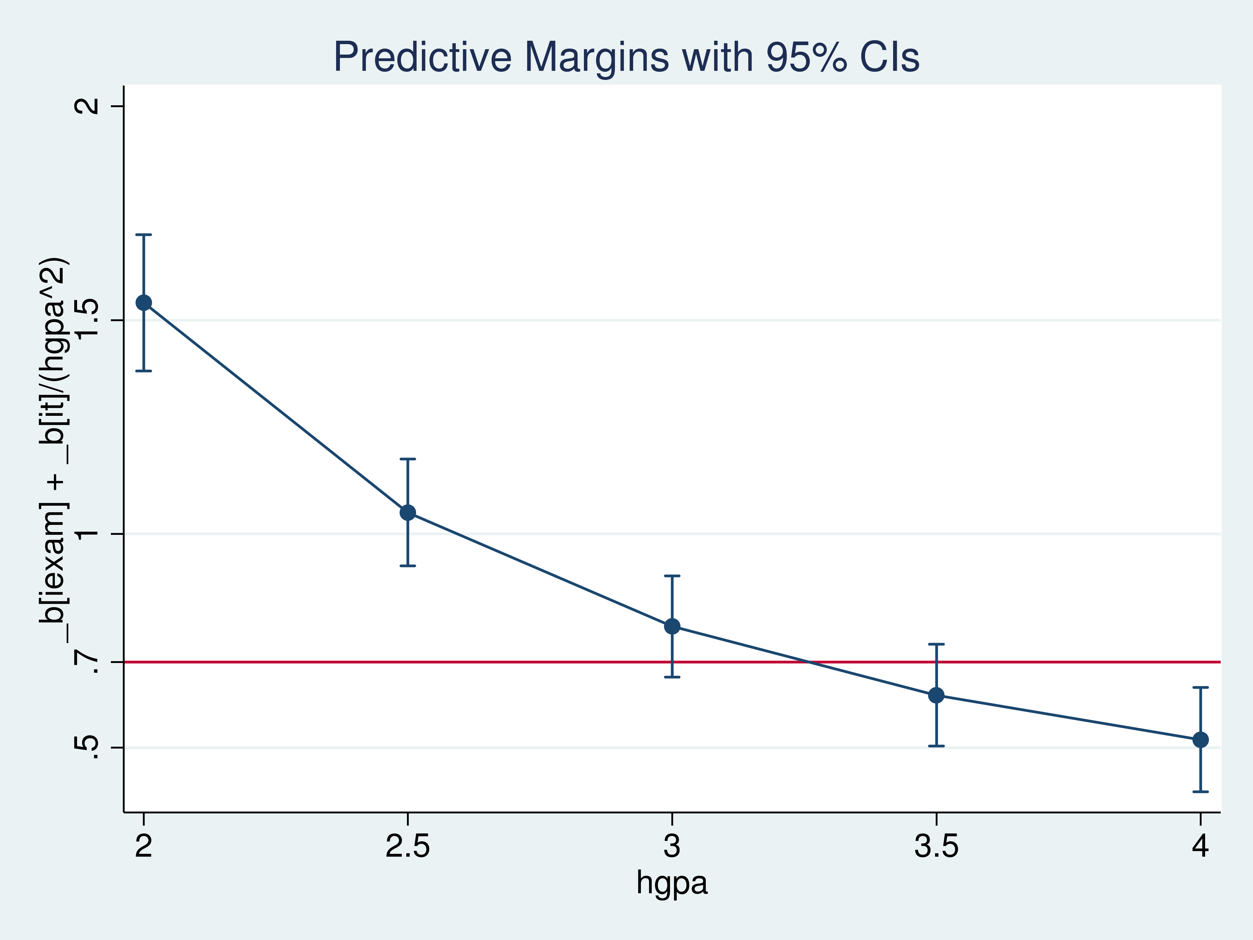
I couldn’t rule out the likelihood {that a} 10-point improve in iexam would trigger a rise of 0.7 within the common csuccess for a pupil with an hgpa of three.5.
Think about the case by which (Eb[y|x,{bf z}]) is my regression mannequin for the end result (y) as a operate of (x), whose impact I need to estimate, and ({bf z}), that are different variables on which I situation. The regression operate (Eb[y|x,{bf z}]) tells me the imply of (y) for given values of (x) and ({bf z}).
The distinction between the imply of (y) given (x_1) and ({bf z}) and the imply of (y) given (x_0) and ({bf z}) is an impact of (x), and it’s given by (Eb[y|x=x_1,{bf z}] – Eb[y|x=x_0,{bf z}]). This impact can fluctuate with ({bf z}); it is likely to be scientifically and statistically vital for some values of ({bf z}) and never for others.
Beneath the same old assumption of right specification, I can estimate the parameters of (Eb[y|x,{bf z}]) utilizing regress or one other command. I can then use margins and marginsplot to estimate results of (x). (I additionally incessantly use lincom, nlcom, and predictnl to estimate results of (x) for given ({bf z}) values.)
Inhabitants-averaged results after regress
Returning to the instance, as a substitute of being a counselor, suppose that I’m a college administrator who believes that assigning sufficient tutors to the course will elevate every pupil’s iexam rating by 10 factors. I start through the use of margins to estimate the typical college-success rating that’s noticed when every pupil will get his or her present iexam rating and to estimate the typical college-success rating that will be noticed when every pupil will get an additional 10 factors on his or her iexam rating.
Instance 5: The common of csuccess with present iexam scores and when every pupil will get an additional 10 factors
. margins, at(iexam = generate(iexam))
>         at(iexam = generate(iexam+1) it = generate((iexam+1)/(hgpa^2)))

Predictive margins                            Variety of obs     =      1,000
Mannequin VCE    : Sturdy

Expression   : Linear prediction, predict()

1._at        : iexam           = iexam

2._at        : iexam           = iexam+1
               it              = (iexam+1)/(hgpa^2)

----------------------------------------------------------------------------
           |            Delta-method
           |     Margin   Std. Err.      t    P>|t|     [95% Conf. Interval]
-----------+----------------------------------------------------------------
       _at |
        1  |   20.76273   .0434416   477.95   0.000     20.67748    20.84798
        2  |   21.48141   .0744306   288.61   0.000     21.33535    21.62747
----------------------------------------------------------------------------
Simply to be sure that I perceive what margins is doing, I compute the typical of the anticipated values when every pupil will get his or her present iexam rating and when every pupil will get an additional 10 factors on his or her iexam rating.
Instance 6: The common of csuccess with present iexam scores and when every pupil will get an additional 10 factors (hand calculations)
. protect

. predict double yhat0
(choice xb assumed; fitted values)

. substitute iexam       = iexam + 1
(1,000 actual modifications made)

. substitute it          = (iexam)/(hgpa^2)
(1,000 actual modifications made)

. predict double yhat1
(choice xb assumed; fitted values)

. summarize yhat0 yhat1

    Variable |      Obs        Imply    Std. Dev.       Min        Max
-------------+-------------------------------------------------------
       yhat0 |    1,000    20.76273    1.625351   17.33157   26.56351
       yhat1 |    1,000    21.48141    1.798292   17.82295   27.76324

. restore
As anticipated, the typical of the predictions for yhat0 match these reported by margins for _at.1, and the typical of the predictions for yhat1 match these reported by margins for _at.2.
Now that I perceive what margins is doing, I take advantage of the distinction choice to estimate the distinction between the typical of csuccess when every pupil will get an additional 10 factors and the typical of csuccess when every pupil will get his or her authentic rating.
Instance 7: The distinction within the averages of csuccess when every pupil will get an additional 10 factors and with present scores
. margins, at(iexam = generate(iexam))
>         at(iexam = generate(iexam+1) it = generate((iexam+1)/(hgpa^2)))
>         distinction(atcontrast(r._at) nowald)

Contrasts of predictive margins
Mannequin VCE    : Sturdy

Expression   : Linear prediction, predict()

1._at        : iexam           = iexam

2._at        : iexam           = iexam+1
               it              = (iexam+1)/(hgpa^2)

--------------------------------------------------------------
             |            Delta-method
             |   Distinction   Std. Err.     [95% Conf. Interval]
-------------+------------------------------------------------
         _at |
   (2 vs 1)  |   .7186786   .0602891      .6003702     .836987
--------------------------------------------------------------
The usual error in instance 7 is labeled as “Delta-method”, which implies that it takes the covariate observations as fastened and accounts for the parameter estimation error. Holding the covariate observations as fastened will get me inference for this specific batch of scholars. I add the choice vce(unconditional) in instance 8, as a result of I would like inference for the inhabitants from which I can repeatedly draw samples of scholars.
Instance 8: The distinction within the averages of csuccess with an unconditional commonplace error
. margins, at(iexam = generate(iexam))
>         at(iexam = generate(iexam+1) it = generate((iexam+1)/(hgpa^2)))
>         distinction(atcontrast(r._at) nowald) vce(unconditional)

Contrasts of predictive margins

Expression   : Linear prediction, predict()

1._at        : iexam           = iexam

2._at        : iexam           = iexam+1
               it              = (iexam+1)/(hgpa^2)

--------------------------------------------------------------
             |            Unconditional
             |   Distinction   Std. Err.     [95% Conf. Interval]
-------------+------------------------------------------------
         _at |
   (2 vs 1)  |   .7186786   .0609148      .5991425    .8382148
--------------------------------------------------------------
On this case, the usual error for the pattern impact reported in instance 7 is about the identical as the usual error for the inhabitants impact reported in instance 8. With actual knowledge, the distinction in these commonplace errors tends to be larger.
Recall the case by which (Eb[y|x,{bf z}]) is my regression mannequin for the end result (y) as a operate of (x), whose impact I need to estimate, and ({bf z}), that are different variables on which I situation. The distinction between the imply of (y) given (x_1) and the imply of (y) given (x_0) is an impact of (x) that has been averaged over the distribution of ({bf z}),
[
Eb[y|x=x_1] – Eb[y|x=x_0] = Eb_{bf Z}left[ Eb[y|x=x_1,{bf z}]proper] –
Eb_{bf Z}left[ Eb[y|x=x_0,{bf z}]proper]
]
Beneath the same old assumptions of right specification, I can estimate the parameters of (Eb[y|x,{bf z}]) utilizing regress or one other command. I can then use margins and marginsplot to estimate a imply of those results of (x). The pattern should be consultant, maybe after weighting, to ensure that the estimated imply of the consequences to converge to a inhabitants imply.
Accomplished and undone
The change in a regression operate that outcomes from an everything-else-held-equal change in a covariate defines an impact of a covariate. I illustrated that when a covariate enters the regression operate nonlinearly, the impact varies over covariate values, inflicting the conditional-on-covariate impact to vary from the population-averaged impact. I additionally confirmed how one can estimate and interpret these conditional-on-covariate and population-averaged results.