Discrete Diffusion: Steady-Time Markov Chains

Could 22, 2025

This put up, supposed to be the primary in a collection associated to discrete diffusion fashions, has been sitting in my drafts for months. I believed that Google’s launch of Gemini Diffusion could be a superb event to lastly publish it.

Whereas discrete time Markov chains – sequences of random variables through which the previous and future are impartial given the current – are moderately well-known in machine studying, fewer individuals ever come throughout their steady cousins. On condition that these fashions function in work on discrete diffusion fashions (see e.g. Lou et al, 2023, Sahoo et al, 2024, Shi et al, 2024, clearly not a whole listing), I believed it might be a great way to get again to running a blog by writing about these fashions – and who is aware of, perhaps keep it up writing a collection about discrete diffusion. For now, the objective of this put up is that will help you construct some key instinct about how continuous-time MCs work.

A Markov chain is a stochastic course of (infinite assortment of random variables listed by time $t$) outlined by two properties:

• the random variables take discrete values (we name them states), and
• the method is memory-less: What occurs to the method sooner or later solely relies on the state it’s in in the mean time. Mathematically, $X_{u} perp X_s vert X_t$ for all $s > t > u$, the place $perp$ denotes conditional independence.

We differentiate Markov chains on values the index $t$ can take: if $t$ is an integer, we name it a discrete-time Markov chain, and when $t$ is actual, we name the method a continuous-time Markov chain.

Discrete Markov chains are totally described by a set of state transition matrices $P_t = [P(X_{t+1} = ivert X_{t}=j)]{i,j}$. Observe that this matrix $P_t$ is listed by the point $t$, as it may possibly, on the whole, change over time. If $P_t = P$ is fixed, we name the Markov chain homogeneous.

Steady time homogeneous chains

To increase the notion of MC to steady time, we’re first going to develop an alternate mannequin of a discrete chains, by contemplating ready occasions in a homogeneous discrete-time Markov chain. Ready occasions are the time the chain spends in the identical state earlier than transitioning to a different state. If the MC is homogeneous, then in each timestep it has a hard and fast likelihood $p_{i,i}$ of staying there. The ready time due to this fact follows a geometric distribution with parameter $p_{i,i}$.

The geometric distribution is the one discrete distribution with the memory-less property, said as $mathbb{P}[T=s+tvert T>s] = mathbb{P}[T = t]$. What this implies is: if you’re at time s, and you recognize the occasion hasn’t occurred but, the distribution of the remaining ready time is identical, no matter how lengthy you’ve got been ready. It seems, the geometric distribution is the one discrete distribution with this property.

With this statement, we will alternatively describe a homogeneous discrete-time Markov chain when it comes to ready occasions, and leap possibilities as follows. Ranging from state $i$ the Markov chain:

• stays in the identical state for a time drawn from a Geometric distribution with parameter $p_{i,i}$
• when the ready time expires, we pattern a brand new state $i neq j$ with likelihood $frac{p_{i,j}}{sum_{kneq i} p_{i,okay}}$

In different phrases, we have now decomposed the outline of the Markov chain when it comes to when the subsequent leap occurs, and the way the state modifications when the leap occurs. On this illustration, if we wish one thing like a Markov chain in steady time, we will try this by permitting the ready time to take actual, not simply integer, values. We will do that by changing the geometric distribution by a steady likelihood distribution. To protect the Markov property, nevertheless, it will be important that we protect the memoryless property $mathbb{P}[T=s+tvert T>s] = mathbb{P}[T = t]$. There is just one such steady distribution: the exponential distribution. A homogeneneous continuous-time Markov chain is thus described as follows. Ranging from state $i$ at time $t$:

• keep in the identical state for a time drawn from an exponential distribution with some parameter $lambda_{i,i}$
• when the ready time expires, pattern a brand new state $i neq j$ with likelihood $frac{lambda_{i,j}}{sum_{kneq i} lambda_{i,okay}}$

Discover that I launched a brand new set of parameters $lambda_{i,j}$ which now changed the transition possibilities $p_{i,j}$. These not should be likelihood distributions, they simply should be all optimistic actual values. The matrix containing these parameters will likely be referred to as the speed matrix, which I’ll denote by $Lambda$, however I will notice that in current machine studying papers, they usually use the notation $Q$ for the speed matrix.

Non-homogeneous Markov chains and level processes

The above description solely actually works for homogeneous Markov chains, through which the ready time distribution doesn’t change over time. When the transition possibilities can change over time, the wait time can not be described as exponential, and it is truly not so trivial to generalise to steady time on this method. To do this, we want one more various view on how Markov chains work: we as a substitute contemplate their relationship to level processes.

Level processes

Think about the next state of affairs which is able to illustrate the connection between the discrete uniform, the Bernoulli, the binomial and the geometric distributions.

The Easter Bunny is hiding eggs in 50 meter lengthy (one dimensional) backyard. In each 1 meter phase he hides at most one egg. He needs to guarantee that on common, there’s a 10% probability of an egg in every 1 meter phase, and he additionally needs the eggs to seem random.

Bunny is contemplating a number of other ways of reaching this:

Course of 1: Bunny steps from sq. to sq.. At each sq., he hides an egg with likelihood 0.1, and passes to the subsequent sq..

bernoulli = partial(numpy.random.binomial, n=1)
backyard = ['_']*50

for i in vary(50):
  if bernoulli(0.1)
    backyard[i] = '🥚'

print(''.be a part of(backyard))

>>> __________🥚__🥚______🥚_🥚__________________🥚________

Course of 2: At every step Bunny attracts a random non-negative integer $T$ from a Geometric distribution with parameter 0.1. He then strikes T cells to the appropriate. If he’s nonetheless inside bounds of the backyard, he hides an egg the place he’s, and repeats the method till he’s out of bounds.

backyard = ['_']*50
bunny_pos = -1

whereas bunny_pos<50: 
  bunny_pos += geometric(0.1)
  if bunny_pos<50:
    backyard[bunny_pos] = '🥚'

print(''.be a part of(backyard))

>>> 🥚______🥚_________________🥚______________🥚🥚🥚___🥚_🥚🥚

Course of 3: Bunny first decides what number of eggs he will disguise in whole within the backyard. Then he samples random areas (with out alternative) from throughout the backyard, and hides an egg at these areas:

backyard = ['_']*50
number_of_eggs = binomial(p=0.1, n=50)
random_locations = permutation(np.arange(50))[:number_of_eggs]

for location in random_locations:
  backyard[location] = '🥚'

print(''.be a part of(backyard))

>>> ________🥚_____🥚_______________🥚_🥚______🥚________🥚🥚

It seems it doesn’t matter which of those processes Bunny follows, on the finish of the day, the end result (binary string representing presence or absence of eggs) follows the identical distribution.

What Bunny does in every of those processes, is he simulated a discrete-time level course of with parameter $p=0.1$. All these numerous processes are equal representations of the purpose course of:

• a binary sequence the place every digit is sampled from impartial Bernoulli
• a binary sequence the place the hole between 1s follows a geometrical distribution
• a binary sequence the place the variety of 1s follows a binomial distribution, and the areas of 1s observe a uniform distribution (with the constraint that they aren’t equal).

Steady level processes

And this egg-hiding course of does have a steady restrict, one the place the backyard will not be subdivided into 50 segments, however is as a substitute handled as a steady phase alongside which eggs might seem anyplace. Like good physicists – and horrible dad and mom – do, we’ll contemplate point-like Easter eggs which have measurement $0$ and may seem arbitrarily shut to one another.

Whereas course of 1 appears inherently discrete (it loops over enumerable areas) each Course of 2 and Course of 3 will be made steady, by changing the discrete likelihood distributions with steady cousins.

• In Course of 2 we change the geometric with the, additionally memoryless, exponential.
• In Course of 3 we change the binomial with its limiting Poisson distribution, and the uniform sampling with out alternative by a steady uniform distribution over the house. We will drop the constraint that the areas should be completely different, since this holds with probabilty one for steady distributions.

In each instances, the gathering of random areas we find yourself with is what is called a homogeneous Poisson level course of. As an alternative of a likelihood $p$, this course of will now have a optimistic parameter $lambda$ that controls the anticipated variety of factors the method goes to position within the interval.

Level processes and Markov Chains

Again to Markov chains. How are level processes and Markov chains associated? The looks of exponential and geometric distributions in Course of 2 of producing level processes could be a giveaway, the ready occasions within the Markov chains will likely be associated to the ready occasions between subsequent factors in a random level course of. Right here is how we will use level processes to simulate a Markov chain. Ranging from the discrete case let’s denote by $p_{i,j}$ the transition likelihood from state $i$ to state $j$

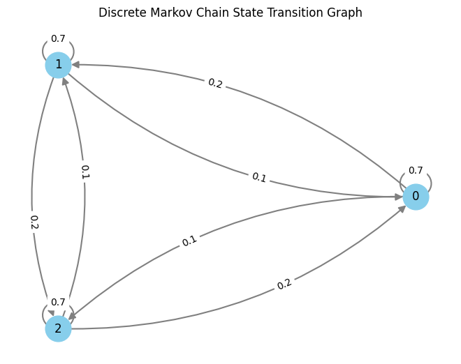
Step 1: For every of the $N(N-1)$ attainable transitions $i rightarrow j$ between $N$ states, draw an impartial level processes with parameter $p_{i,j}$. We now have an inventory of of occasion occasions for every transition. These will be visualised for a three-state Markov Chain as follows:

This plot has one line for every transition from a state $i$ to a different state $j$. For every of those we drew transition factors from some extent course of. Discover how among the strains are denser – it’s because the corresponding transition possibilities are increased. That is the transition matrix I used:

To show this set of level processes right into a Markov chain, we have now to repeat the next steps ranging from time 0.

Assume at time $t$ the Markov chain is in state $i$. We contemplate the purpose processes for all transitions out of state $i$, and take a look at the earliest occasion in any of those sequences that occur after time $t$. Suppose this earlier occasion is at time $s+t$ and occurs within the level course of we drew for transition $i rightarrow j$. Our course of will then keep in state $i$ till time $s+t$, then we leap to to state $j$ and repeat the method.

That is illustrated within the following determine:

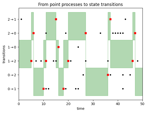
We begin the Markov chain in state $1$. We due to this fact give attention to the transitions $1rightarrow 0$ and $1 rightarrow 2$, as highlighted by the inexperienced space on the left aspect of this determine. We keep in state $1$ till we encounter a transition occasion (black dot) for both of those two transitions. This occurs after about 5 timesteps, as illustrated by the purple cross. At this level, we transition to state $2$, for the reason that first transition occasion was noticed within the $1 rightarrow 2$ row. Now we give attention to transition occasions for strains $2rightarrow 1$ and $2rightarrow 0$, i.e. the highest two rows. We do not have to attend too lengthy till a transition occasion is noticed, triggering a state replace to state $0$, and so forth. You’ll be able to learn off the Markov chain states from the place the inexperienced focus space lies.

This reparametrisation of a CTMC when it comes to underlying Poisson level processes now opens the door for us to simulate non-homogeneous CTMCs as properly. However, as this put up is already fairly lengthy, I am not going to let you know right here the right way to do it. Let that be your homework to consider: Return to course of 2 and course of 3 of simulating the homogeneous Poisson course of. Take into consideration what makes them homogeneous (i.e. the identical over time)? Which parts would change if the speed matrix wasn’t fixed over time? Which illustration can deal with non-constant charges extra simply?

Abstract

On this put up I tried to convey some essential, and I believe cool, instinct about steady time Markov chains. I focussed on exploring completely different representations of a Markov chain, every of which recommend a distinct method of simulating or sampling from the identical course of. Here’s a recap of some key concepts mentioned:

• You’ll be able to reparametrise a homogeneous discrete Markov chain when it comes to ready occasions sampled from a geometrical distribution, and transition possibilities.
• The geometric distribution has a memory-less property which has a deep reference to the Markov property of Markov chains.
• One option to go steady is to contemplate a steady ready time distribution which preserves the memorylessness: the exponential distribution. This gave us our first illustration of a continuous-time chain, however it’s tough to increase this to non-homogeneous case the place the speed matrix might change over time.
• We then mentioned completely different representations of discrete level processes, and famous (though didn’t show) their equivalence.
• We may contemplate steady variations of those level processes, by changing discrete distributions by steady ones, once more preserving essential options comparable to memorylessness.
• We additionally mentioned how a Markov chain will be described when it comes to underlying level processes: every state pair has an related level course of, and transitions occur when some extent course of related to the present state “fires”.
• This was a redundant illustration of the Markov chain, inasmuch as most factors sampled from the underlying level processes didn’t contribute to the state evolution in any respect (within the final figures, most black dots lie exterior the inexperienced space, so you possibly can transfer their areas with out effecting the states of the chain).