

In grad college I specialised in differential equations, however by no means labored with delay-differential equations, equations specifying {that a} answer relies upon not solely on its derivatives but in addition on the state of the operate at a earlier time. The primary time I labored with a delay-differential equation would come a pair many years later once I did some modeling work for a pharmaceutical firm.
Massive delays can change the qualitative conduct of a differential equation, however it appears believable that sufficiently delays shouldn’t. That is right, and we’ll present simply how small “small enough” is in a easy particular case. We’ll take a look at the equation
x′(t) = a x(t) + b x(t − τ)
the place the coefficients a and b are non-zero actual constants and the delay τ is a optimistic fixed. Then [1] proves that the equation above has the identical qualitative conduct as the identical equation with the delay eliminated, i.e. with τ = 0, supplied τ is sufficiently small. Right here “sufficiently small” means
−1/e < bτ exp(−aτ) < e
and
aτ < 1.
There’s a additional speculation for the theory cited above, a technical situation that holds on a nowhere dense set. The answer to a primary order delay-differential just like the one we’re taking a look at right here isn’t decided by an preliminary situation x(0) = x0 alone. We’ve got to specify the answer over the interval [−τ, 0]. This may be any operate of t, topic solely to a technical situation that holds on a nowhere-dense set of preliminary situations. See [1] for particulars.
Instance
Let’s take a look at a selected instance,
x′(t) = −3 x(t) + 2 x(t − τ)
with the preliminary situation x(1) = 1. If there have been no delay time period τ, the answer could be x(t) = exp(1 − t). On this case the answer monotonically decays to zero.
The concept above says we should always anticipate the identical conduct so long as
−1/e < 2τ exp(3τ) < e
which holds so long as τ < 0.404218.
Let’s remedy our equation for the case τ = 0.4 utilizing Mathematica.
tau = 0.4
answer = NDSolveValue[
    {x'[t] == -3 x[t] + 2 x[t - tau], x[t /; t <= 1] == t },
    x, {t, 0, 10}]
Plot[solution[t], {t, 0, 10}, PlotRange -> All]
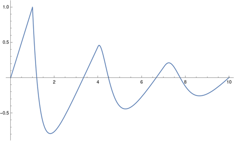
This produces the next plot.
The answer initially ramps as much as 1, as a result of that’s what we specified, however evidently finally the answer monotonically decays to 0, simply as when τ = 0.
After we change the delay to τ = 3 and rerun the code we get oscillations.
[1] R. D. Driver, D. W. Sasser, M. L. Slater. The Equation x’ (t) = ax (t) + bx (t – τ) with “Small” Delay. The American Mathematical Month-to-month, Vol. 80, No. 9 (Nov., 1973), pp. 990–995