

In my final publish, I confirmed you easy methods to create a desk of statistical assessments utilizing the command() choice within the new and improved desk command. On this publish, I’ll present you easy methods to collect data and create tables utilizing the brand new acquire suite of instructions. Our objective is to suit three logistic regression fashions and create the desk within the Adobe PDF doc beneath.
Create the fundamental desk
Let’s start by typing webuse nhanes2l to open the NHANES dataset after which typing describe to look at a few of the variables.
. webuse nhanes2l
(Second Nationwide Well being and Vitamin Examination Survey)

. describe highbp age intercourse diabetes

Variable      Storage   Show    Worth
    title         kind    format    label      Variable label
-------------------------------------------------------------------------------
highbp          byte    %8.0g               * Hypertension
age             byte    %9.0g                 Age (years)
intercourse             byte    %9.0g      intercourse        Intercourse
diabetes        byte    %12.0g     diabetes   Diabetes standing
The dataset contains age, intercourse, an indicator for hypertension (highbp), and an indicator for diabetes (diabetes).
A brand new technique for constructing tables
We are going to match three logistic regression fashions for the binary end result highbp. For every mannequin, we’ll use the logistic command to estimate the chances ratios and customary errors. Then we’ll use estat ic to estimate the Akaike’s data criterion (AIC) and Schwarz’s Bayesian data criterion (BIC) for every mannequin. Our last desk will embrace data for 3 fashions from six totally different instructions.
Given the relative complexity of our desk, we’re going to use a brand new technique to construct it. We are going to use acquire get to collect data from every command. Then we’ll use acquire structure to outline the structure of our desk. Let’s do a easy instance for example this technique earlier than we start the complete desk.
Let’s kind acquire get: earlier than our first logistic regression command.
. acquire get: logistic highbp c.age i.intercourse

Logistic regression                                    Variety of obs =  10,351
                                                       LR chi2(2)    = 1563.54
                                                       Prob > chi2   =  0.0000
Log chance = -6268.9975                            Pseudo R2     =  0.1109

------------------------------------------------------------------------------
      highbp | Odds ratio   Std. err.      z    P>|z|     [95% conf. interval]
-------------+----------------------------------------------------------------
         age |   1.049042   .0013945    36.02   0.000     1.046313    1.051779
             |
         intercourse |
     Feminine  |    .648767   .0280172   -10.02   0.000     .5961141    .7060706
       _cons |   .0887874   .0063561   -33.83   0.000     .0771641    .1021615
------------------------------------------------------------------------------
Notice: _cons estimates baseline odds.
Subsequent let’s kind acquire structure to outline the structure of a desk with row dimension colname and column dimension outcome. I’ve used sq. brackets to incorporate solely the degrees _r_b and _r_se from the dimension outcome. This can add columns for the coefficients and customary errors, respectively.
. acquire structure (colname) (outcome[_r_b _r_se])

Assortment: default
      Rows: colname
   Columns: outcome[_r_b _r_se]
   Desk 1: 4 x 2

------------------------------------
            | Coefficient Std. error
------------+-----------------------
Age (years) |    1.049042   .0013945
Male        |           1          0
Feminine      |     .648767   .0280172
Intercept   |    .0887874   .0063561
------------------------------------
That was straightforward! We created a fundamental desk of regression output with two instructions. The output tells us that acquire get created a brand new assortment named default.
Let’s repeat this technique and add some choices. Let’s start by typing acquire clear to clear any collections from Stata’s reminiscence. Then let’s use acquire create to create a brand new assortment named MyModels.
acquire clear
acquire create MyModels
Subsequent let’s use the acquire get choice title() to collect the outcomes from our logistic regression mannequin in our assortment named MyModels. Notice that I’ve typed acquire slightly than acquire get. The phrase “get” just isn’t obligatory.
acquire, title(MyModels): logistic highbp c.age i.intercourse
I might additionally wish to specify a brand new dimension and degree for the outcomes of my logistic regression mannequin. I can do that utilizing the tag() choice. The fundamental syntax is tag(dimension[level]). The instance beneath shops the outcomes of the logistic regression mannequin to the extent (1) within the dimension mannequin.
acquire, title(MyModels)                    ///
        tag(mannequin[(1)])                    ///
        : logistic highbp c.age i.intercourse
The instance above shops all the outcomes from the mannequin. However we’ll solely want the coefficients and customary errors. We will specify an inventory of outcomes to be mechanically reported within the desk by together with these outcomes after acquire. The instance beneath collects solely the coefficients (_r_b) and the usual errors (_r_se) from the logistic regression mannequin.
acquire _r_b _r_se,                    ///
        title(MyModels)                 ///
        tag(mannequin[(1)])                ///
        : logistic highbp c.age i.intercourse
Now we will use acquire structure to create a desk from the outcomes we saved in degree (1) of dimension mannequin within the assortment MyTables.
. acquire structure (colname#outcome) (mannequin[(1)]), title(MyModels)

Assortment: MyModels
      Rows: colname#outcome
   Columns: mannequin[(1)]
   Desk 1: 12 x 1

------------------------
              |      (1)
--------------+---------
Age (years)   |
  Coefficient | 1.049042
  Std. error  | .0013945
Male          |
  Coefficient |        1
  Std. error  |        0
Feminine        |
  Coefficient |  .648767
  Std. error  | .0280172
Intercept     |
  Coefficient | .0887874
  Std. error  | .0063561
------------------------
You could be questioning how I chosen the row and column dimensions for acquire structure. I might clarify why this specific instance labored. However it could not work to your tables. So let’s stroll by the steps I used to determine it out.
Some particulars about acquire structure
Let’s start by typing acquire dims to view an inventory of the size in our assortment.
. acquire dims

Assortment dimensions
Assortment: MyModels
-----------------------------------------
                   Dimension   No. ranges
-----------------------------------------
Structure, model, header, label
                      cmdset   1
                       coleq   1
                     colname   8
           colname_remainder   1
                       mannequin   1
               program_class   1
                      outcome   43
                 result_type   3
                     rowname   1
                         intercourse   2

Fashion solely
                border_block   4
                   cell_type   4
-----------------------------------------
The dimension outcome catches my eye due to the title and since it has 43 ranges. We will view an inventory of the degrees by typing acquire levelsof outcome.
. acquire levelsof outcome

Assortment: MyModels
 Dimension: outcome
    Ranges: N N_cdf N_cds _r_b _r_ci _r_df _r_lb _r_p _r_se _r_ub _r_z chi2
            chi2type cmd cmdline converged depvar df_m estat_cmd ic okay k_dv
            k_eq k_eq_model ll ll_0 marginsnotok marginsok ml_method mns choose p
            predict properties r2_p rank rc guidelines approach title person vce
            which
The dimension outcome comprises estimates of the coefficients, customary errors, and lots of different statistical outcomes from our mannequin. Let’s use acquire structure to create a desk for the dimension outcome.
. acquire structure (outcome), title(MyModels)

Assortment: MyModels
      Rows: outcome

Your structure specification doesn't uniquely match any objects. Dimension colname
would possibly assist uniquely match objects.
That didn’t work. However the output means that together with the dimension colname would possibly assist. The dimension named colname has eight ranges and we will view an inventory of the degrees by typing acquire levelsof colname.
. acquire levelsof colname

Assortment: MyModels
 Dimension: colname
    Ranges: age 1.intercourse 2.intercourse c1 c2 c3 c4 _cons
The dimension colname contains the variable names, together with issue variables, from our logistic regression mannequin. It additionally comprises ranges named c1, c2, c3, and c4. Let’s add the row dimension colname and see what occurs.
. acquire structure (colname) (outcome), title(MyModels)

Assortment: MyModels
      Rows: colname
   Columns: outcome
   Desk 1: 4 x 2

------------------------------------
            | Coefficient Std. error
------------+-----------------------
Age (years) |    1.049042   .0013945
Male        |           1          0
Feminine      |     .648767   .0280172
Intercept   |    .0887874   .0063561
That labored—we’ve a desk! However the desk raises an vital query. The dimension outcome has 43 ranges, and the dimension colname included ranges like c1. Why aren’t all of these ranges displayed within the desk?
The reply is that acquire structure solely contains cells the place there’s a worth related to every degree of each the row and the column dimensions. Recall that we requested that solely the coefficients (_r_b) and customary errors (_r_se) from our mannequin be displayed. And people coefficients and customary errors had been solely collected for the degrees age, 1.intercourse, 2.intercourse, and _cons for the dimension colname.
As soon as we perceive this idea, we will discover different layouts for our desk. For instance, we might stack the coefficients and customary errors underneath every variable in our mannequin.
. acquire structure (colname#outcome) (), title(MyModels)

Assortment: MyModels
      Rows: colname#outcome
   Desk 1: 12 x 1

------------------------
Age (years)   |
  Coefficient | 1.049042
  Std. error  | .0013945
Male          |
  Coefficient |        1
  Std. error  |        0
Feminine        |
  Coefficient |  .648767
  Std. error  | .0280172
Intercept     |
  Coefficient | .0887874
  Std. error  | .0063561
------------------------
We are going to ultimately create an analogous column of outcomes for every of those three fashions. Recall that we created the dimension mannequin with acquire, tag(). Let’s view the degrees of the dimension mannequin by typing acquire levelsof mannequin.
. acquire levelsof mannequin

Assortment: MyModels
 Dimension: mannequin
    Ranges: (1)
For now, the dimension mannequin has one degree named (1), and we will specify mannequin as our column dimension.
. acquire structure (colname#outcome) (mannequin[(1)]), title(MyModels)

Assortment: MyModels
      Rows: colname#outcome
   Columns: mannequin[(1)]
   Desk 1: 12 x 1

------------------------
              |      (1)
--------------+---------
Age (years)   |
  Coefficient | 1.049042
  Std. error  | .0013945
Male          |
  Coefficient |        1
  Std. error  |        0
Feminine        |
  Coefficient |  .648767
  Std. error  | .0280172
Intercept     |
  Coefficient | .0887874
  Std. error  | .0063561
------------------------
This method to constructing tables in steps could be useful in case you are not sure easy methods to start. Begin by typing acquire dims to view the size within the assortment. Then use acquire levelsof to view the degrees of every dimension. Then experiment with acquire structure to design your desk. The output of acquire structure will usually present useful directions.
Amassing outcomes from a number of instructions
Recall that we might additionally like to incorporate the AIC and BIC for every mannequin in our desk, and we will estimate them by typing estat ic after we match the mannequin.
. estat ic

Akaike's data criterion and Bayesian data criterion

-----------------------------------------------------------------------------
       Mannequin |          N   ll(null)  ll(mannequin)      df        AIC        BIC
-------------+---------------------------------------------------------------
           . |     10,351  -7050.765  -6268.998       3      12544   12565.73
-----------------------------------------------------------------------------
Notice: BIC makes use of N = variety of observations. See [R] BIC be aware.
The estimates of the AIC and BIC are saved in a matrix named r(S).
. return record

matrices:
                  r(S) :  1 x 6
And we will view the matrix by typing matlist r(S).
. matlist r(S)

             |         N        ll0         ll         df        AIC        BIC
-------------+------------------------------------------------------------------
           . |     10351  -7050.765  -6268.998          3      12544   12565.73
We will check with the AIC and BIC within the matrix r(S) utilizing matrix subscripting. The final syntax to check with a component in a matrix is matname[row,column]. Utilizing this syntax, we will check with the BIC as r(S)[1,6]. Column 6 is called BIC, so we will additionally check with the BIC as r(S)[1,”BIC”].
. show r(S)[1,"BIC"]
12565.73
Let’s acquire the AIC and BIC and retailer them in degree (1) of dimension mannequin in our MyModels assortment.
acquire AIC=r(S)[1,"AIC"]    ///
        BIC=r(S)[1,"BIC"],   ///
        title(MyModels)       ///
        tag(mannequin[(1)])      ///
        : estat ic
Then we will embrace them in our desk by including outcome[AIC BIC] to the row dimension of acquire structure.
. acquire structure (colname#outcome outcome[AIC BIC]) (mannequin[(1)]), title(MyModels)

Assortment: MyModels
      Rows: colname#outcome outcome[AIC BIC]
   Columns: mannequin[(1)]
   Desk 1: 14 x 1

------------------------
              |      (1)
--------------+---------
Age (years)   |
  Coefficient | 1.049042
  Std. error  | .0013945
Male          |
  Coefficient |        1
  Std. error  |        0
Feminine        |
  Coefficient |  .648767
  Std. error  | .0280172
Intercept     |
  Coefficient | .0887874
  Std. error  | .0063561
AIC           |    12544
BIC           | 12565.73
------------------------
Discover that I didn’t embrace the “#” operator after I added the row dimension outcome[AIC BIC]. It’s because AIC and BIC are usually not nested inside every degree of the dimension colname. I merely needed so as to add rows for AIC and BIC on the backside of the desk.
Including extra fashions to the desk
Let’s add a second mannequin to our desk. Discover that the instructions beneath are almost equivalent to the instructions I used above. There are solely two variations. First, I’ve used factor-variable notation so as to add the interplay of age and intercourse to the logistic regression mannequin. And second, I’m storing the outcomes to degree (2) of the dimension mannequin.
acquire _r_b _r_se,                    ///
        title(MyModels)                 ///
        tag(mannequin[(2)])                ///
        : logistic highbp c.age##i.intercourse

acquire AIC=r(S)[1,"AIC"]              ///
        BIC=r(S)[1,"BIC"],             ///
        title(MyModels)                 ///
        tag(mannequin[(2)])                ///
        : estat ic
We will use acquire structure to be sure that it labored.
. acquire structure (colname#outcome outcome[AIC BIC]) (mannequin), title(MyModels)

Assortment: MyModels
      Rows: colname#outcome outcome[AIC BIC]
   Columns: mannequin
   Desk 1: 20 x 2

----------------------------------------
                     |      (1)      (2)
---------------------+------------------
Age (years)          |
  Coefficient        | 1.049042 1.035184
  Std. error         | .0013945 .0018459
Male                 |
  Coefficient        |        1        1
  Std. error         |        0        0
Feminine               |
  Coefficient        |  .648767 .1556985
  Std. error         | .0280172 .0224504
Male # Age (years)   |
  Coefficient        |                 1
  Std. error         |                 0
Feminine # Age (years) |
  Coefficient        |          1.028811
  Std. error         |           .002794
Intercept            |
  Coefficient        | .0887874 .1690035
  Std. error         | .0063561 .0153794
AIC                  |    12544 12434.34
BIC                  | 12565.73 12463.32
----------------------------------------
That labored, so let’s add a 3rd mannequin to our desk. Let’s add the variable diabetes to our second mannequin. And we’ll retailer the outcomes to degree (3) of the dimension mannequin.
acquire _r_b _r_se,                         ///
        title(MyModels)                      ///
        tag(mannequin[(3)])                     ///
        : logistic highbp c.age##i.intercourse i.diabetes

acquire AIC=r(S)[1,"AIC"]                   ///
        BIC=r(S)[1,"BIC"],                  ///
        title(MyModels)                      ///
        tag(mannequin[(3)])                     ///
        : estat ic
Let’s use acquire structure once more to be sure that it labored.
. acquire structure (colname#outcome outcome[AIC BIC]) (mannequin), title(MyModels)

Assortment: MyModels
      Rows: colname#outcome outcome[AIC BIC]
   Columns: mannequin
   Desk 1: 26 x 3

-------------------------------------------------
                     |      (1)      (2)      (3)
---------------------+---------------------------
Age (years)          |
  Coefficient        | 1.049042 1.035184 1.034281
  Std. error         | .0013945 .0018459 .0018566
Male                 |
  Coefficient        |        1        1        1
  Std. error         |        0        0        0
Feminine               |
  Coefficient        |  .648767 .1556985 .1549363
  Std. error         | .0280172 .0224504 .0223461
Male # Age (years)   |
  Coefficient        |                 1        1
  Std. error         |                 0        0
Feminine # Age (years) |
  Coefficient        |          1.028811 1.028856
  Std. error         |           .002794 .0027958
Not diabetic         |
  Coefficient        |                          1
  Std. error         |                          0
Diabetic             |
  Coefficient        |                   1.521011
  Std. error         |                    .154103
Intercept            |
  Coefficient        | .0887874 .1690035 .1730928
  Std. error         | .0063561 .0153794 .0157789
AIC                  |    12544 12434.34 12417.74
BIC                  | 12565.73 12463.32 12453.97
-------------------------------------------------
Now we’ve the fundamental structure of our desk. All we have to do now’s customise the structure and export it to an Adobe PDF doc.
Use acquire model to format the desk
I’ll use acquire model showbase, acquire model row, acquire model cell, and acquire model header to customise the structure of our desk. The instructions within the code block beneath are the identical instructions I utilized in earlier posts, so I gained’t clarify every step right here. However I’ve included feedback to refresh our reminiscence.
// TURN OFF BASE LEVELS FOR FACTOR VARIABLES
acquire model showbase off
// CHANGE THE INTERACTION DELIMITER
acquire model row stack, spacer delimiter(" x ")
// REMOVE THE VERTICAL LINE
acquire model cell border_block, border(proper, sample(nil))
// FORMAT THE NUMBERS
acquire model cell, nformat(%5.2f)
acquire model cell outcome[AIC BIC], nformat(%8.0f)
// PUT PARENTHESES AROUND THE STANDARD ERRORS
acquire model cell outcome[_r_se], sformat("(%s)")
// LABEL AIC AND BIC
acquire model header outcome[AIC BIC], degree(label)
Let’s kind acquire preview to verify our work up to now.
. acquire preview

-----------------------------------------
                        (1)    (2)    (3)
-----------------------------------------
Age (years)
  Coefficient          1.05   1.04   1.03
  Std. error         (0.00) (0.00) (0.00)

Feminine
  Coefficient          0.65   0.16   0.15
  Std. error         (0.03) (0.02) (0.02)

Feminine x Age (years)
  Coefficient                 1.03   1.03
  Std. error                (0.00) (0.00)

Diabetic
  Coefficient                        1.52
  Std. error                       (0.15)

Intercept
  Coefficient          0.09   0.17   0.17
  Std. error         (0.01) (0.02) (0.02)

AIC                   12544  12434  12418

BIC                   12566  12463  12454
-----------------------------------------
Subsequent I’ll use some choices which are distinctive to this desk. First, I’ll use the acquire model cell choice halign() to middle the objects and column headers within the desk.
. acquire model cell cell_type[item column-header], halign(middle)

. acquire preview

-----------------------------------------
                       (1)    (2)    (3)
-----------------------------------------
Age (years)
  Coefficient         1.05   1.04   1.03
  Std. error         (0.00) (0.00) (0.00)

Feminine
  Coefficient         0.65   0.16   0.15
  Std. error         (0.03) (0.02) (0.02)

Feminine x Age (years)
  Coefficient                1.03   1.03
  Std. error                (0.00) (0.00)

Diabetic
  Coefficient                       1.52
  Std. error                       (0.15)

Intercept
  Coefficient         0.09   0.17   0.17
  Std. error         (0.01) (0.02) (0.02)

AIC                   12544  12434  12418

BIC                   12566  12463  12454
-----------------------------------------
Then I’ll use the acquire model header choice degree() to cover the labels for the row dimension outcome.
. acquire model header outcome, degree(conceal)

. acquire preview

-----------------------------------------
                       (1)    (2)    (3)
-----------------------------------------
Age (years)           1.05   1.04   1.03
                     (0.00) (0.00) (0.00)

Feminine                0.65   0.16   0.15
                     (0.03) (0.02) (0.02)

Feminine x Age (years)         1.03   1.03
                            (0.00) (0.00)

Diabetic                            1.52
                                   (0.15)

Intercept             0.09   0.17   0.17
                     (0.01) (0.02) (0.02)

AIC                   12544  12434  12418

BIC                   12566  12463  12454
-----------------------------------------
And eventually, I’ll use the acquire model column choice extraspace so as to add an additional area between the columns. I feel this makes it simpler to learn the desk.
. acquire model column, extraspace(1)

. acquire preview

----------------------------------------------
                        (1)      (2)      (3)
----------------------------------------------
Age (years)            1.05     1.04     1.03
                      (0.00)   (0.00)   (0.00)

Feminine                 0.65     0.16     0.15
                      (0.03)   (0.02)   (0.02)

Feminine x Age (years)            1.03     1.03
                               (0.00)   (0.00)

Diabetic                                 1.52
                                        (0.15)

Intercept              0.09     0.17     0.17
                      (0.01)   (0.02)   (0.02)

AIC                    12544    12434    12418

BIC                    12566    12463    12454
----------------------------------------------
We did it! We collected the outcomes from our fashions and customised the structure.
Export the desk to an Adobe PDF doc
I confirmed you easy methods to export your tables to a Microsoft Phrase doc in my earlier posts. Let’s attempt one thing new and export our desk to an Adobe PDF doc. Many of the putpdf instructions are equivalent to their corresponding putdocx instructions, with the plain exception that they start with putpdf slightly than putdocx. However there are a couple of vital variations.
First, I’ve changed putdocx paragraph, model() with putpdf paragraph, font() halign(). The primary occasion units the font to a 26-point Calibri Gentle font and facilities the textual content horizonally on the web page. The second occasion units the font to a 14-point Calibri Gentle font and begins the textual content on the left of the web page. The third occasion doesn’t specify a font() or halign() choice, so the default 11-point Helvetica font is used.
Second, I’ve changed the acquire model putdocx choice structure(autofitcontents) with the acquire model putpdf choices width() and indent(). The width(60%) choice units the width of the desk to 60% of the complete width of the web page. The indent(1 in) choice indents the desk one inch from the left aspect of the web page.
And third, I’ve used the be aware() choice with acquire model putpdf so as to add a be aware to the desk to inform the reader that the desk shows odds ratios with customary errors in parentheses.
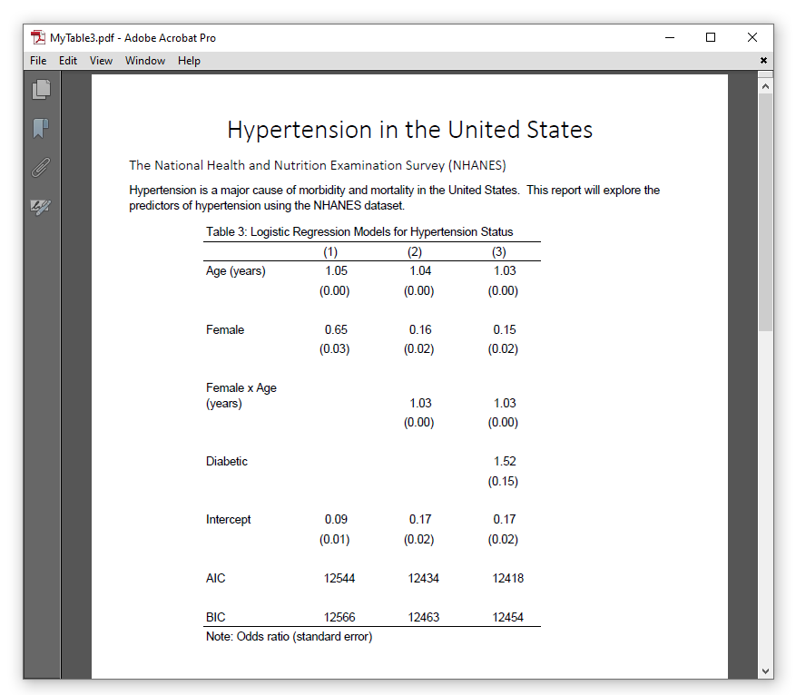
putpdf clear
putpdf start
putpdf paragraph, font("Calibri Gentle",26) halign(middle)
putpdf textual content ("Hypertension in the USA")
putpdf paragraph, font("Calibri Gentle",14) halign(left)
putpdf textual content ("The Nationwide Well being and Vitamin Examination Survey (NHANES)")
putpdf paragraph
putpdf textual content ("Hypertension is a significant explanation for morbidity and mortality in ")
putpdf textual content ("the USA.  This report will discover the predictors ")
putpdf textual content ("of hypertension utilizing the NHANES dataset.")
acquire model putpdf, width(60%) indent(1 in)                                ///
        title("Desk 3: Logistic Regression Fashions for Hypertension Standing") ///
        be aware("Notice: Odds ratio (customary error)")
putpdf acquire
putpdf save MyTable3.pdf, exchange
The ensuing Adobe PDF doc seems to be just like the picture beneath.
Conclusion
On this publish, we realized a brand new technique to create tables utilizing solely the acquire suite of instructions. We used acquire get to gather outcomes from Stata instructions, and we used acquire structure to specify the structure of our desk. We realized easy methods to title our collections and retailer the outcomes from instructions to particular ranges of dimensions.
You might have most likely seen that we’ve used the identical set of acquire model instructions in these weblog posts. We might proceed to repeat and paste them into our future do-files, however there may be a better method to reuse acquire model instructions. In my subsequent publish, I’ll present you easy methods to use acquire model save and acquire model use to save lots of kinds and reuse them with different tables. And I’ll present you easy methods to use acquire label save and acquire label use to save lots of labels for the degrees of dimensions.