

In my final submit, I confirmed you the right way to use the brand new and improved desk command with the command() choice to create a desk of statistical assessments. On this submit, I need to present you the right way to use the command() choice to create a desk for a single regression mannequin. Our aim is to create the desk within the Microsoft Phrase doc beneath.
Create the fundamental desk
Let’s start by typing webuse nhanes2l to open the NHANES dataset, and let’s kind describe to look at a few of the variables.
. webuse nhanes2l
(Second Nationwide Well being and Diet Examination Survey)

. describe highbp age intercourse diabetes

Variable      Storage   Show    Worth
    identify         kind    format    label      Variable label
-------------------------------------------------------------------------------
highbp          byte    %8.0g               * Hypertension
age             byte    %9.0g                 Age (years)
intercourse             byte    %9.0g      intercourse        Intercourse
diabetes        byte    %12.0g     diabetes   Diabetes standing
The dataset consists of age, intercourse, an indicator for hypertension (highbp), and an indicator for diabetes (diabetes). We want to match a logistic regression mannequin for the binary consequence highbp and create a desk of the percentages ratios, commonplace errors, z statistics, p-values, and confidence intervals. Word that I’ve used Stata’s factor-variable notation within the instance beneath to incorporate the principle impact of the continual variable age, the principle impact of the specific variables intercourse and diabetes, and the interplay of age and intercourse.
. logistic highbp c.age##i.intercourse i.diabetes

Logistic regression                                    Variety of obs =  10,349
                                                       LR chi2(4)    = 1691.59
                                                       Prob > chi2   =  0.0000
Log probability = -6203.8722                            Pseudo R2     =  0.1200

------------------------------------------------------------------------------
      highbp | Odds ratio   Std. err.      z    P>|z|     [95% conf. interval]
-------------+----------------------------------------------------------------
         age |   1.034281   .0018566    18.78   0.000     1.030648    1.037926
             |
         intercourse |
     Feminine  |   .1549363   .0223461   -12.93   0.000     .1167849    .2055511
             |
   intercourse#c.age |
     Feminine  |   1.028856   .0027958    10.47   0.000     1.023391    1.034351
             |
    diabetes |
   Diabetic  |   1.521011    .154103     4.14   0.000     1.247073    1.855124
       _cons |   .1730928   .0157789   -19.24   0.000      .144772    .2069537
------------------------------------------------------------------------------
Word: _cons estimates baseline odds.
Let’s start by putting the logistic regression command within the command() possibility of a desk command. There are not any row dimensions, and the column dimensions are command and end result.
. desk () (command end result),
>          command(logistic highbp c.age##i.intercourse i.diabetes)

-----------------------------------------------------------------------
                             |  logistic highbp c.age##i.intercourse i.diabetes
-----------------------------+-----------------------------------------
Age (years)                  |                                 1.034281
Intercourse=Male                     |                                        1
Intercourse=Feminine                   |                                 .1549363
Intercourse=Male # Age (years)       |                                        1
Intercourse=Feminine # Age (years)     |                                 1.028856
Diabetes standing=Not diabetic |                                        1
Diabetes standing=Diabetic     |                                 1.521011
Intercept                    |                                 .1730928
-----------------------------------------------------------------------
By default, the desk shows the coefficients, which are literally odds ratios as a result of we used the logistic command.
desk robotically created a group named Desk, and we will view the scale by typing accumulate dims.
. accumulate dims

Assortment dimensions
Assortment: Desk
-----------------------------------------
                   Dimension   No. ranges
-----------------------------------------
Format, model, header, label
                      cmdset   1
                       coleq   2
                     colname   13
           colname_remainder   2
                     command   1
                    diabetes   2
               program_class   1
                      end result   43
                 result_type   3
                       roweq   1
                     rowname   2
                         intercourse   2
                     statcmd   1

Model solely
                border_block   4
                   cell_type   4
-----------------------------------------
The dimension end result has 43 ranges. Let’s kind accumulate label checklist to view the degrees and their labels.
. accumulate label checklist end result, all

  Assortment: Desk
   Dimension: end result
       Label: End result
Stage labels:
           N  Variety of observations
       N_cdf  Variety of utterly decided failures
       N_cds  Variety of utterly decided successes
        _r_b  Coefficient
       _r_ci  __LEVEL__% CI
       _r_df  df
       _r_lb  __LEVEL__% decrease sure
        _r_p  p-value
       _r_se  Std. error
       _r_ub  __LEVEL__% higher sure
        _r_z  z
       (output omitted)
We have an interest within the ranges that start with _r, so I’ve omitted a lot of the output. The degrees that start with _r are the contents of the desk of coefficients. For instance, the extent _r_b comprises coefficients (that’s, odds ratios), the extent _r_se comprises the usual errors, and so forth. Word that the boldness interval is saved in a single degree, _r_ci, and likewise in separate ranges for the higher and decrease bounds, _r_lb and r_ub, respectively.
Let’s add the percentages ratio, commonplace error, and confidence interval to our desk by together with _r_b _r_se _r_ci to our command() possibility. We’ll add the z take a look at and p-value later.
. desk () (command end result),
>          command(_r_b _r_se _r_ci
>                  : logistic highbp c.age##i.intercourse i.diabetes)

-------------------------------------------------------------------------------
                             |      logistic highbp c.age##i.intercourse i.diabetes
                             |  Coefficient   Std. error          95% CI
-----------------------------+-------------------------------------------------
Age (years)                  |     1.034281     .0018566   1.030648    1.037926
Intercourse=Male                     |            1            0
Intercourse=Feminine                   |     .1549363     .0223461   .1167849    .2055511
Intercourse=Male # Age (years)       |            1            0
Intercourse=Feminine # Age (years)     |     1.028856     .0027958   1.023391    1.034351
Diabetes standing=Not diabetic |            1            0
Diabetes standing=Diabetic     |     1.521011      .154103   1.247073    1.855124
Intercept                    |     .1730928     .0157789    .144772    .2069537
-------------------------------------------------------------------------------
Subsequent let’s customise the show of the numbers in our desk. I’ve used nformat() to show the percentages ratios, commonplace errors, and condidence interval with two digits to the suitable of the decimal. I’ve used sformat() to position sq. brackets across the confidence interval, and I’ve used cidelimiter() to position a comma between the decrease and higher bounds of the boldness interval.
. desk () (command end result),
>          command(_r_b _r_se _r_ci
>                  : logistic highbp c.age##i.intercourse i.diabetes)
>          nformat(%5.2f  _r_b _r_se _r_ci )
>          sformat("[%s]"  _r_ci )
>          cidelimiter(,)

---------------------------------------------------------------------------
                             |    logistic highbp c.age##i.intercourse i.diabetes
                             |    Coefficient    Std. error       95% CI
-----------------------------+---------------------------------------------
Age (years)                  |           1.03          0.00    [1.03, 1.04]
Intercourse=Male                     |           1.00          0.00
Intercourse=Feminine                   |           0.15          0.02    [0.12, 0.21]
Intercourse=Male # Age (years)       |           1.00          0.00
Intercourse=Feminine # Age (years)     |           1.03          0.00    [1.02, 1.03]
Diabetes standing=Not diabetic |           1.00          0.00
Diabetes standing=Diabetic     |           1.52          0.15    [1.25, 1.86]
Intercept                    |           0.17          0.02    [0.14, 0.21]
---------------------------------------------------------------------------
The column of odds ratios is labeled Coefficient, and we will change it to Odds Ratio utilizing accumulate label ranges.
. accumulate label ranges end result _r_b "Odds Ratio", modify

. accumulate preview

---------------------------------------------------------------------------
                             |    logistic highbp c.age##i.intercourse i.diabetes
                             |    Odds Ratio     Std. error       95% CI
-----------------------------+---------------------------------------------
Age (years)                  |          1.03           0.00    [1.03, 1.04]
Intercourse=Male                     |          1.00           0.00
Intercourse=Feminine                   |          0.15           0.02    [0.12, 0.21]
Intercourse=Male # Age (years)       |          1.00           0.00
Intercourse=Feminine # Age (years)     |          1.03           0.00    [1.02, 1.03]
Diabetes standing=Not diabetic |          1.00           0.00
Diabetes standing=Diabetic     |          1.52           0.15    [1.25, 1.86]
Intercept                    |          0.17           0.02    [0.14, 0.21]
---------------------------------------------------------------------------
The dimension command has one degree that’s labeled with our logistic regression command. We are able to additionally modify its label utilizing accumulate label ranges.
. accumulate label ranges command 1
>          "Logistic Regression Mannequin for Hypertension", modify

. accumulate preview

------------------------------------------------------------------------------
                             |    Logistic Regression Mannequin for Hypertension
                             |     Odds Ratio      Std. error       95% CI
-----------------------------+------------------------------------------------
Age (years)                  |           1.03            0.00     [1.03, 1.04]
Intercourse=Male                     |           1.00            0.00
Intercourse=Feminine                   |           0.15            0.02     [0.12, 0.21]
Intercourse=Male # Age (years)       |           1.00            0.00
Intercourse=Feminine # Age (years)     |           1.03            0.00     [1.02, 1.03]
Diabetes standing=Not diabetic |           1.00            0.00
Diabetes standing=Diabetic     |           1.52            0.15     [1.25, 1.86]
Intercept                    |           0.17            0.02     [0.14, 0.21]
------------------------------------------------------------------------------
By default, desk shows the bottom degree, also called the ‘referent class’ or ‘referent group’, of issue variables. For instance, the row labeled Intercourse=Male is the bottom degree for the issue variable i.intercourse. The class Male is used within the denominator of the percentages ratio. We are able to cover the bottom ranges of all issue variables, together with interactions, by typing accumulate model showbase off.
. accumulate model showbase off

. accumulate preview

--------------------------------------------------------------------------
                         |    Logistic Regression Mannequin for Hypertension
                         |     Odds Ratio      Std. error       95% CI
-------------------------+------------------------------------------------
Age (years)              |           1.03            0.00     [1.03, 1.04]
Intercourse=Feminine               |           0.15            0.02     [0.12, 0.21]
Intercourse=Feminine # Age (years) |           1.03            0.00     [1.02, 1.03]
Diabetes standing=Diabetic |           1.52            0.15     [1.25, 1.86]
Intercept                |           0.17            0.02     [0.14, 0.21]
--------------------------------------------------------------------------
Subsequent let’s use accumulate model row to customise the row labels. By default, the variables and classes are displayed aspect by aspect with a “binder” character. For instance, Intercourse=Feminine shows the variable Intercourse adopted by the binder = adopted by the class Feminine. The choice stack shows the variable identify as soon as after which shows every class beneath the variable identify. The choice nobinder removes the binder character, =. Interactions are displayed utilizing the # character and we will use the delimiter(” x “) possibility to alter the interplay delimiter to x.
. accumulate model row stack, nobinder delimiter(" x ")

. accumulate preview

-------------------------------------------------------------------
                  |    Logistic Regression Mannequin for Hypertension
                  |     Odds Ratio      Std. error       95% CI
------------------+------------------------------------------------
Age (years)       |           1.03            0.00     [1.03, 1.04]
Intercourse               |
  Feminine          |           0.15            0.02     [0.12, 0.21]
Intercourse x Age (years) |
  Feminine          |           1.03            0.00     [1.02, 1.03]
Diabetes standing   |
  Diabetic        |           1.52            0.15     [1.25, 1.86]
Intercept         |           0.17            0.02     [0.14, 0.21]
-------------------------------------------------------------------
We eliminated the vertical line from the tables in my earlier posts, and we will do the identical factor right here utilizing accumulate model cell to take away the suitable border from the primary column.
. accumulate model cell border_block, border(proper, sample(nil))

. accumulate preview

-----------------------------------------------------------------
                     Logistic Regression Mannequin for Hypertension
                      Odds Ratio      Std. error       95% CI
-----------------------------------------------------------------
Age (years)                 1.03            0.00     [1.03, 1.04]
Intercourse
  Feminine                    0.15            0.02     [0.12, 0.21]
Intercourse x Age (years)
  Feminine                    1.03            0.00     [1.02, 1.03]
Diabetes standing
  Diabetic                  1.52            0.15     [1.25, 1.86]
Intercept                   0.17            0.02     [0.14, 0.21]
-----------------------------------------------------------------
We might cease right here and export our desk to a Microsoft Phrase doc. However chances are you’ll want to embody columns for the z statistic and the p-value in your desk. I’ve added these columns within the code block beneath utilizing the degrees _r_z and _r_p.
desk () (command end result),                          ///
command(_r_b _r_se _r_z _r_p _r_ci                  ///
: logistic highbp c.age##i.intercourse i.diabetes)          ///
nformat(%5.2f  _r_b _r_se _r_ci )                   ///
nformat(%5.4f  _r_p)                                ///
sformat("[%s]"  _r_ci )                             ///
cidelimiter(,)

accumulate label ranges end result _r_b "Odds Ratio", modify
accumulate label ranges command 1 "Logistic Regression Mannequin for Hypertension", modify
accumulate model showbase off
accumulate model row stack, delimiter(" x ") nobinder
accumulate model cell border_block, border(proper, sample(nil))
. accumulate preview
----------------------------------------------------------------------------
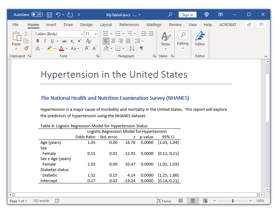
Logistic Regression Mannequin for Hypertension
Odds Ratio Std. error z p-value 95% CI
----------------------------------------------------------------------------
Age (years) 1.03 0.00 18.78 0.0000 [1.03, 1.04]
Intercourse
Feminine 0.15 0.02 -12.93 0.0000 [0.12, 0.21]
Intercourse x Age (years)
Feminine 1.03 0.00 10.47 0.0000 [1.02, 1.03]
Diabetes standing
Diabetic 1.52 0.15 4.14 0.0000 [1.25, 1.86]
Intercept 0.17 0.02 -19.24 0.0000 [0.14, 0.21]
----------------------------------------------------------------------------
And now we will export our closing desk to a Microsoft Phrase doc utilizing putdocx.
putdocx clear
putdocx start
putdocx paragraph, model(Title)
putdocx textual content ("Hypertension in the USA")
putdocx paragraph, model(Heading1)
putdocx textual content ("The Nationwide Well being and Diet Examination Survey (NHANES)")
putdocx paragraph
putdocx textual content ("Hypertension is a significant reason for morbidity and mortality in ")
putdocx textual content ("the USA.  This report will discover the predictors ")
putdocx textual content ("of hypertension utilizing the NHANES dataset.")
accumulate model putdocx, format(autofitcontents)               ///
title("Desk 4: Logistic Regression Mannequin for Hypertension Standing")
putdocx accumulate
putdocx save MyTable4.docx, change
Conclusion
On this submit, we realized the right way to use the command() possibility with the desk command to create a desk from a logistic regression mannequin. The steps can be almost similar for different regression fashions resembling linear regression or probit regression.
First, specify the column dimensions column and end result. Second, choose the columns, resembling _r_b and _r_ci, then place your regression command within the command() possibility. Then customise the show of the row and column labels and the numbers as you would like.
I’ll present you the right way to use accumulate to create a desk for a number of regression fashions in my subsequent submit.