

Right this moment, I’m going to start a sequence of weblog posts about customizable tables in Stata 17. We expanded the performance of the desk command. We additionally developed a wholly new system that lets you accumulate outcomes from any Stata command, create customized desk layouts and types, save and use these layouts and types, and export your tables to hottest doc codecs. We even added a new handbook to indicate you find out how to use this highly effective and versatile system.
I need to present you a number of examples earlier than I present you find out how to create your personal customizable tables. I’ll present you find out how to re-create these examples in future posts.
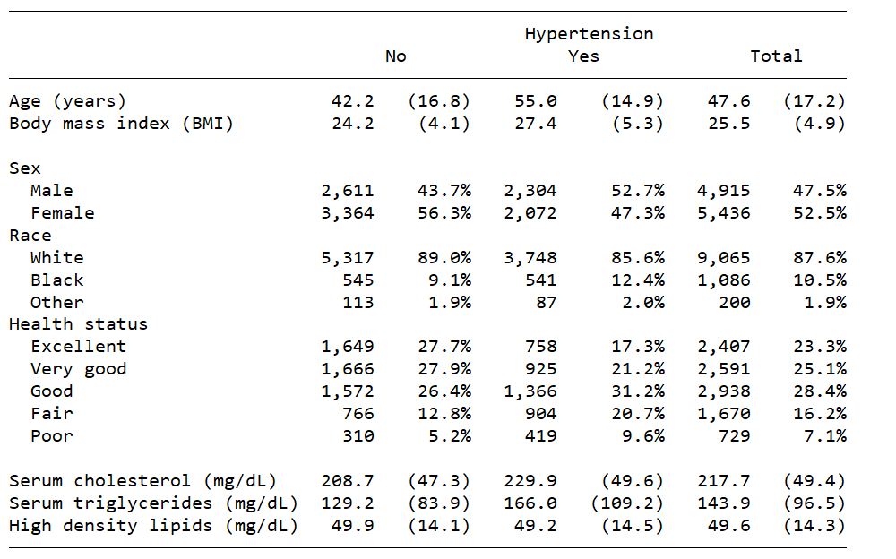
The traditional desk 1
The primary instance is a traditional “desk 1”. Most studies and papers start with a desk of descriptive statistics for the pattern that’s usually subdivided by a categorical variable. The desk beneath studies means and customary deviations for steady variables and exhibits frequencies and percentages for categorical variables. These statistics are displayed for every class of hypertension and all the pattern.
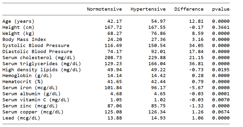
Desk of statistical check outcomes
Generally, we want to report a proper speculation check for a gaggle of variables. The desk beneath studies the means for a gaggle of steady variables for contributors with out hypertension, with hypertension, the distinction between the means, and the p-value for a t check.
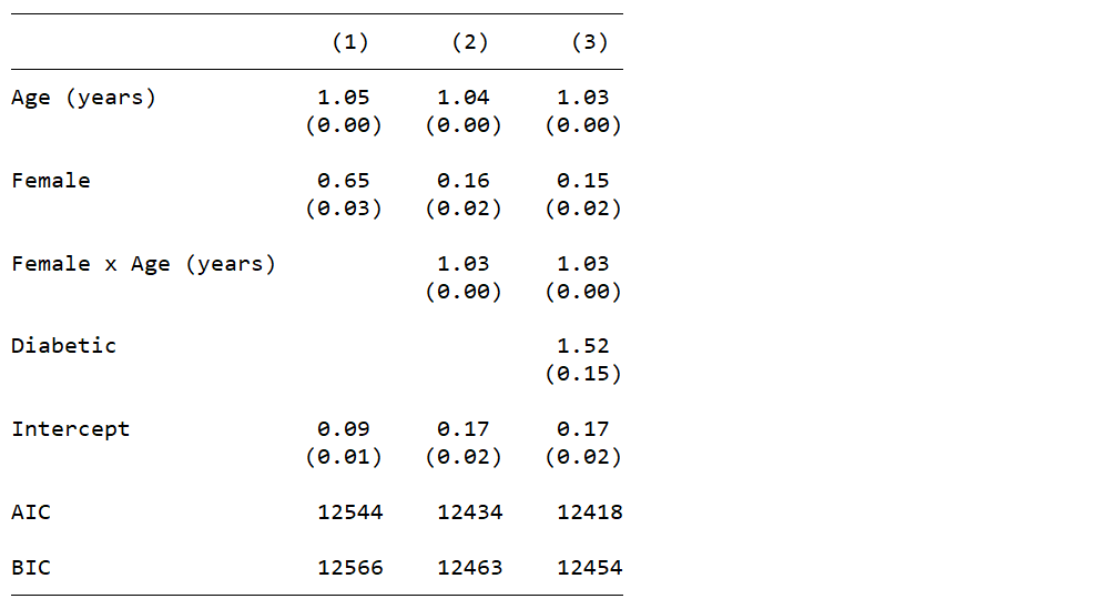
Desk for a number of regression fashions
We may additionally want to create a desk to check the outcomes of a number of regression fashions. The desk beneath shows the chances ratios and customary errors for the covariates of three logistic regression fashions together with the AIC and BIC for every mannequin.
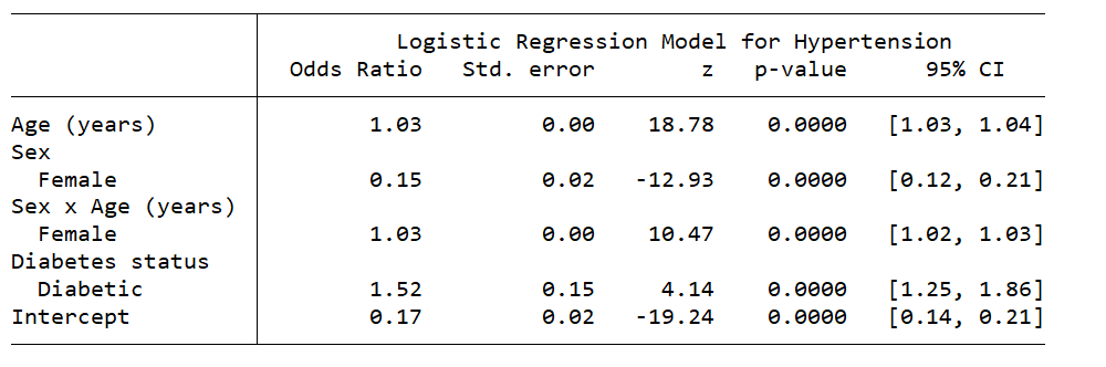
Desk for a single regression mannequin
We may additionally want to show the outcomes of our remaining regression mannequin. The desk beneath shows the chances ratio, customary error, z rating, p-value, and 95% confidence interval for every covariate in our remaining mannequin.
Chances are you’ll desire a special structure on your tables, and that’s the level of this sequence of weblog posts. My objective is to indicate you find out how to create your personal custom-made tables and import them into your paperwork.
The info
Let’s start by typing webuse nhanes2l to open a dataset that incorporates information from the Nationwide Well being and Vitamin Examination Survey (NHANES), and let’s describe a number of the variables we’ll be utilizing.
. webuse nhanes2l
(Second Nationwide Well being and Vitamin Examination Survey)

. describe age intercourse race peak weight bmi highbp
>          bpsystol bpdiast tcresult tgresult hdresult

Variable      Storage   Show    Worth
    identify         kind    format    label      Variable label
------------------------------------------------------------------------------------------------------------------------
age             byte    %9.0g                 Age (years)
intercourse             byte    %9.0g      intercourse        Intercourse
race            byte    %9.0g      race       Race
peak          float   %9.0g                 Top (cm)
weight          float   %9.0g                 Weight (kg)
bmi             float   %9.0g                 Physique mass index (BMI)
highbp          byte    %8.0g               * Hypertension
bpsystol        int     %9.0g                 Systolic blood stress
bpdiast         int     %9.0g                 Diastolic blood stress
tcresult        int     %9.0g                 Serum ldl cholesterol (mg/dL)
tgresult        int     %9.0g                 Serum triglycerides (mg/dL)
hdresult        int     %9.0g                 Excessive density lipids (mg/dL)
This dataset incorporates demographic, anthropometric, and organic measures for contributors in the US. We are going to ignore the survey weights for now in order that we will concentrate on the syntax for creating tables.
Introduction to the desk command
The fundamental syntax of desk is desk (RowVars) (ColVars). The instance beneath creates a desk for the row variable highbp.
. desk (highbp) ()

--------------------------------
                    |  Frequency
--------------------+-----------
Hypertension |
  0                 |      5,975
  1                 |      4,376
  Complete             |     10,351
--------------------------------
By default, the desk shows the frequency for every class of highbp and the full frequency. The second set of empty parentheses on this instance is just not needed as a result of there isn’t any column variable.
The instance beneath creates a desk for the column variable highbp. The primary set of empty parentheses is critical on this instance in order that desk is aware of that highbp is a column variable.
. desk () (highbp)

------------------------------------
          |    Hypertension
          |       0       1    Complete
----------+-------------------------
Frequency |   5,975   4,376   10,351
------------------------------------
The instance beneath creates a cross-tabulation for the row variable intercourse and the column variable highbp. The row and column totals are included by default.
. desk (intercourse) (highbp)

-----------------------------------
         |    Hypertension
         |       0       1    Complete
---------+-------------------------
Intercourse      |
  Male   |   2,611   2,304    4,915
  Feminine |   3,364   2,072    5,436
  Complete  |   5,975   4,376   10,351
-----------------------------------
We will take away the row and column totals by together with the nototals choice.
. desk (intercourse) (highbp), nototals

---------------------------------
         |   Hypertension
         |          0           1
---------+-----------------------
Intercourse      |
  Male   |      2,611       2,304
  Feminine |      3,364       2,072
---------------------------------
We will additionally specify a number of row or column variables, or each. The instance beneath shows frequencies for classes of intercourse nested inside classes of highbp.
. desk (highbp intercourse) (), nototals

--------------------------------
                    |  Frequency
--------------------+-----------
Hypertension |
  0                 |
    Intercourse             |
      Male          |      2,611
      Feminine        |      3,364
  1                 |
    Intercourse             |
      Male          |      2,304
      Feminine        |      2,072
--------------------------------
Or we will show frequencies for classes of highbp nested inside classes of intercourse as within the instance beneath. The order of the variables within the parentheses determines the nesting construction within the desk.
. desk (intercourse highbp) (), nototals

------------------------------------
                        |  Frequency
------------------------+-----------
Intercourse                     |
  Male                  |
    Hypertension |
      0                 |      2,611
      1                 |      2,304
  Feminine                |
    Hypertension |
      0                 |      3,364
      1                 |      2,072
------------------------------------
We will specify comparable nesting buildings for a number of column variables. The instance beneath shows frequencies for classes of intercourse nested inside classes of highbp.
. desk () (highbp intercourse), nototals

--------------------------------------------
          |        Hypertension
          |         0                1
          |        Intercourse              Intercourse
          |   Male   Feminine    Male   Feminine
----------+---------------------------------
Frequency |  2,611    3,364   2,304    2,072
--------------------------------------------
Or we will show frequencies for classes of highbp nested inside classes of intercourse as within the instance beneath. Once more, the order of the variables within the parentheses determines the nesting construction within the desk.
. desk () (intercourse highbp), nototals

----------------------------------------------------------
          |                       Intercourse
          |           Male                   Feminine
          |   Hypertension     Hypertension
          |          0           1           0           1
----------+-----------------------------------------------
Frequency |      2,611       2,304       3,364       2,072
----------------------------------------------------------
You possibly can even specify three, or extra, row or column variables. The instance beneath shows frequencies for classes of diabetes nested inside classes of intercourse nested inside classes of highbp.
. desk (highbp intercourse diabetes) (), nototals

------------------------------------
                        |  Frequency
------------------------+-----------
Hypertension     |
  0                     |
    Intercourse                 |
      Male              |
        Diabetes standing |
          Not diabetic  |      2,533
          Diabetic      |         78
      Feminine            |
        Diabetes standing |
          Not diabetic  |      3,262
          Diabetic      |        100
  1                     |
    Intercourse                 |
      Male              |
        Diabetes standing |
          Not diabetic  |      2,165
          Diabetic      |        139
      Feminine            |
        Diabetes standing |
          Not diabetic  |      1,890
          Diabetic      |        182
------------------------------------
The totals() choice
We will embody totals for a specific row or column variable by together with the variable identify within the totals() choice. The choice totals(highbp) within the instance beneath provides totals for the column variable highbp to our desk.
. desk (intercourse) (highbp), totals(highbp)

---------------------------------
         |   Hypertension
         |          0           1
---------+-----------------------
Intercourse      |
  Male   |      2,611       2,304
  Feminine |      3,364       2,072
  Complete  |      5,975       4,376
---------------------------------
The choice totals(intercourse) within the instance beneath provides totals for the row variable intercourse to our desk.
. desk (intercourse) (highbp), totals(intercourse)

-----------------------------------
         |    Hypertension
         |       0        1   Complete
---------+-------------------------
Intercourse      |
  Male   |   2,611    2,304   4,915
  Feminine |   3,364    2,072   5,436
-----------------------------------
We will additionally specify row or column variables for a specific variable even when there are a number of row or column variables. The instance beneath shows totals for the row variable highbp, despite the fact that there are two row variables within the desk.
. desk (intercourse highbp) (), totals(highbp)

------------------------------------
                        |  Frequency
------------------------+-----------
Intercourse                     |
  Male                  |
    Hypertension |
      0                 |      2,611
      1                 |      2,304
  Feminine                |
    Hypertension |
      0                 |      3,364
      1                 |      2,072
  Complete                 |
    Hypertension |
      0                 |      5,975
      1                 |      4,376
------------------------------------
The statistic() choices
Frequencies are displayed by default, however you possibly can specify different statistics with the statistic() choice. For instance, you possibly can show frequencies and percents with the choices statistic(frequency) and statistic(%), respectively.
. desk (intercourse) (highbp),
>       statistic(frequency)
>       statistic(%)
>       nototals

--------------------------------------
              |   Hypertension
              |          0           1
--------------+-----------------------
Intercourse           |
  Male        |
    Frequency |      2,611       2,304
    %   |      25.22       22.26
  Feminine      |
    Frequency |      3,364       2,072
    %   |      32.50       20.02
--------------------------------------
We will additionally embody the imply and customary deviation of age with the choices statistic(imply age) and statistic(sd age), respectively.
. // FORMAT THE NUMBERS IN THE OUTPUT
. desk (intercourse) (highbp),
>       statistic(frequency)
>       statistic(%)
>       statistic(imply age)
>       statistic(sd age)
>       nototals

-----------------------------------------------
                       |   Hypertension
                       |          0           1
-----------------------+-----------------------
Intercourse                    |
  Male                 |
    Frequency          |      2,611       2,304
    %            |      25.22       22.26
    Imply               |    42.8625    52.59288
    Commonplace deviation |    16.9688    15.88326
  Feminine               |
    Frequency          |      3,364       2,072
    %            |      32.50       20.02
    Imply               |   41.62366    57.61921
    Commonplace deviation |   16.59921    13.25577
-----------------------------------------------
You possibly can view a whole record of statistics for the statistic() choice within the Stata handbook.
The nformat() and sformat() choices
We will use the nformat() choice to specify the numerical show format for statistics in our desk. Within the instance beneath, the choice nformat(%9.0fc frequency) shows frequency with commas within the hundreds place and no digits to the fitting of the decimal. The choice nformat(%6.2f imply sd) shows the imply and customary deviation with two digits to the fitting of the decimal.
. desk (intercourse) (highbp),
>       statistic(frequency)
>       statistic(%)
>       statistic(imply age)
>       statistic(sd age)
>       nototals
>       nformat(%9.0fc frequency)
>       nformat(%6.2f  imply sd)

-----------------------------------------------
                       |   Hypertension
                       |          0           1
-----------------------+-----------------------
Intercourse                    |
  Male                 |
    Frequency          |      2,611       2,304
    %            |      25.22       22.26
    Imply               |      42.86       52.59
    Commonplace deviation |      16.97       15.88
  Feminine               |
    Frequency          |      3,364       2,072
    %            |      32.50       20.02
    Imply               |      41.62       57.62
    Commonplace deviation |      16.60       13.26
-----------------------------------------------
We will use the sformat() choice so as to add strings to the statistics in our desk. Within the instance beneath, the choice sformat(“%s%%” %) provides “%” to the statistic %, and the choice sformat(“(%s)” sd) locations parentheses round the usual deviation.
. desk (intercourse) (highbp),
>       statistic(frequency)
>       statistic(%)
>       statistic(imply age)
>       statistic(sd age)
>       nototals
>       nformat(%9.0fc frequency)
>       nformat(%6.2f  imply sd)
>       sformat("%s%%" %)
>       sformat("(%s)" sd)

-----------------------------------------------
                       |   Hypertension
                       |          0           1
-----------------------+-----------------------
Intercourse                    |
  Male                 |
    Frequency          |      2,611       2,304
    %            |     25.22%      22.26%
    Imply               |      42.86       52.59
    Commonplace deviation |    (16.97)     (15.88)
  Feminine               |
    Frequency          |      3,364       2,072
    %            |     32.50%      20.02%
    Imply               |      41.62       57.62
    Commonplace deviation |    (16.60)     (13.26)
-----------------------------------------------
The model() choice
We will use the model() choice to use a predefined model to a desk. Within the instance beneath, the choice model(table-1) applies Stata’s predefined model table-1 to our desk. This model modified the looks of the row labels. You possibly can view a whole record of Stata’s predefined types within the handbook, and I’ll present you find out how to create your personal types in a future weblog submit.
. desk (intercourse) (highbp),
>       statistic(frequency)
>       statistic(%)
>       statistic(imply age)
>       statistic(sd age)
>       nototals
>       nformat(%9.0fc frequency)
>       nformat(%6.2f  imply sd)
>       sformat("%s%%" %)
>       sformat("(%s)" sd)
>       model(table-1)

---------------------------------
         |   Hypertension
         |          0           1
---------+-----------------------
     Intercourse |
  Male   |      2,611       2,304
         |     25.22%      22.26%
         |      42.86       52.59
         |    (16.97)     (15.88)
         |
Feminine   |      3,364       2,072
         |     32.50%      20.02%
         |      41.62       57.62
         |    (16.60)     (13.26)
---------------------------------
Conclusion
We discovered loads in regards to the new-and-improved desk command, however we now have barely scratched the floor. We’ve discovered find out how to create tables and use the nototals, totals(), statistic(), nformat(), sformat(), and model() choices. There are a lot of different choices, and you’ll examine them within the handbook. I’ll present you find out how to use accumulate to customise the looks of your tables in my subsequent submit.
You may as well go to the Stata YouTube Channel to learn to create tables utilizing the desk dialog field and the Tables Builder.
Customizable tables in Stata 17
Customizable tables in Stata 17: Cross-tabulations
Customizable tables in Stata 17: One-way tables of abstract
Customizable tables in Stata 17: Two-way tables of abstract statistics
Customizable tables in Stata 17: Find out how to create tables for a regression mannequin
Customizable tables in Stata 17: Find out how to create tables for a number of regression fashions