

In Stata 17, we launched the brand new gather suite of instructions for creating and customizing tables and the etable command for simply creating and exporting a desk of estimation outcomes. Stata 18 presents one other new command, dtable, that simply builds and exports a desk of descriptive statistics, usually known as Desk 1 in publications. Now producing tables of descriptive statistics for each categorical and steady variables is less complicated than ever. It’s value mentioning that the dual instructions etable and dtable are each constructed on the gather framework we launched in Stata 17, in order that they share plenty of properties.
On this put up, I’ll reveal create and export easy tables of descriptive statistics and extra advanced ones that show statistics by group, check for variations throughout teams, and extra. I
will even present how you should use the gather suite of instructions to additional customise the look of your tables and embody tables created with dtable in full studies.
A easy instance
Earlier than Stata 18, if we needed to generate a desk of descriptive statistics (to be included in a publication later), we would have used summarize to acquire abstract statistics for steady variables and tabulate to report the frequencies, proportions, or percentages for categorical variables. Let’s use auto.dta (1978 car information) to reveal that:
. sysuse auto, clear
(1978 car information)

. summarize value weight mpg

    Variable |        Obs        Imply    Std. dev.       Min        Max
-------------+---------------------------------------------------------
       value |         74    6165.257    2949.496       3291      15906
      weight |         74    3019.459    777.1936       1760       4840
         mpg |         74     21.2973    5.785503         12         41

. tabulate rep78

     Restore |
document 1978 |      Freq.     %        Cum.
------------+-----------------------------------
          1 |          2        2.90        2.90
          2 |          8       11.59       14.49
          3 |         30       43.48       57.97
          4 |         18       26.09       84.06
          5 |         11       15.94      100.00
------------+-----------------------------------
      Whole |         69      100.00
These instructions computed the statistics for us. Nevertheless, manually typing all of those numbers right into a properly formatted desk is tedious work, and it isn’t reproducible when we’ve got new information.
Compared, with dtable, we are able to sort
. dtable value weight mpg i.rep78

----------------------------------------
                          Abstract
----------------------------------------
N                                     74
Worth              6,165.257 (2,949.496)
Weight (lbs.)        3,019.459 (777.194)
Mileage (mpg)             21.297 (5.786)
Restore document 1978
  1                             2 (2.9%)
  2                            8 (11.6%)
  3                           30 (43.5%)
  4                           18 (26.1%)
  5                           11 (15.9%)
----------------------------------------
Simply as straightforward as that, we’ve got constructed a desk exhibiting the pattern measurement of the information, means, and normal deviations for the desired steady variables (value, weight, and mpg), in addition to frequencies and percentages for ranges of the desired categorical variable (rep78).
Along with the outcomes for the complete pattern, we are able to request the above statistics individually for every class of a bunch variable corresponding to international by including the by() choice:
. dtable value weight mpg i.rep78, by(international)

------------------------------------------------------------------------------------
                                               Automotive origin
                          Home              Overseas                Whole
------------------------------------------------------------------------------------
N                             52 (70.3%)            22 (29.7%)           74 (100.0%)
Worth              6,072.423 (3,097.104) 6,384.682 (2,621.915) 6,165.257 (2,949.496)
Weight (lbs.)        3,317.115 (695.364)   2,315.909 (433.003)   3,019.459 (777.194)
Mileage (mpg)             19.827 (4.743)        24.773 (6.611)        21.297 (5.786)
Restore document 1978
  1                             2 (4.2%)              0 (0.0%)              2 (2.9%)
  2                            8 (16.7%)              0 (0.0%)             8 (11.6%)
  3                           27 (56.2%)             3 (14.3%)            30 (43.5%)
  4                            9 (18.8%)             9 (42.9%)            18 (26.1%)
  5                             2 (4.2%)             9 (42.9%)            11 (15.9%)
------------------------------------------------------------------------------------
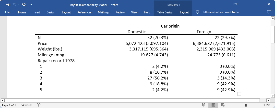
We are able to suppress the column for the whole pattern utilizing the suboption nototal inside by(). And we are able to export the desk to a Phrase doc, myfile.docx, utilizing the choice export():
. dtable value weight mpg i.rep78, by(international, nototal)
> export(myfile.docx, substitute)
(output omitted)
The exported desk appears to be like like
Request custom-made statistics and assessments
By default, dtable studies pattern measurement for the dataset, means and normal deviations for steady variables, and frequencies and percentages for categorical variables. However we are able to request different descriptive statistics corresponding to medians and interquartile ranges. We are able to even specify totally different statistics for various variables in the identical desk. Earlier than we transfer to a extra superior instance, I need to present you the dialog field of dtable.
Go to the menu Statistics > Summaries, tables, and assessments > Desk of descriptive statistics to open the dialog field for dtable.
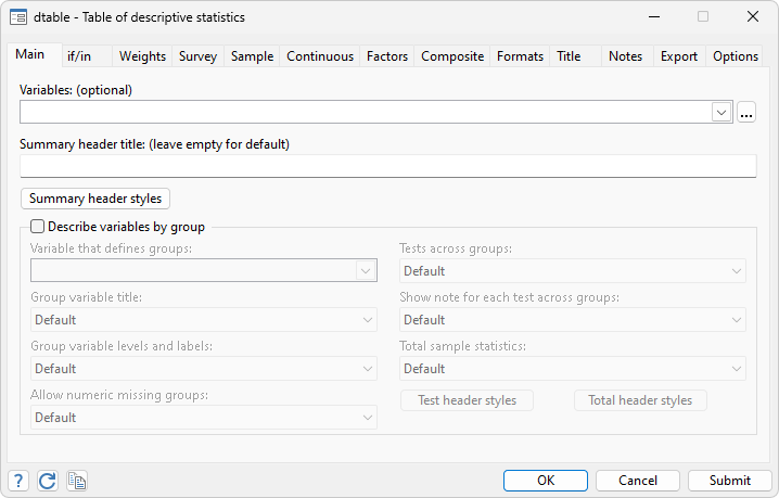
It’s a good suggestion to flick through the tabs within the dialog field to get accustomed to this command. It’s a good way to discover what we are able to do utilizing dtable. I need to spotlight three tabs and go away the others so that you can discover.
- On the Foremost tab, we are able to specify each steady variables and categorical variables of our analysis curiosity (utilizing the i. factor-variable notation to point a categorical variable). We are able to additionally specify the by variable. We are able to management different issues like whether or not we need to present the check end result throughout the by teams, whether or not we need to present the pattern statistics, and so on.
- On the Steady tab, we are able to specify the continual variables (they could or is probably not specified on the Foremost tab), and we are able to request custom-made statistics and assessments for various variables.
- The Elements tab works equally to the Steady tab. We are able to specify issue variables and select custom-made statistics and assessments for various variables there.
For an instance, we’ll load the Modified Bangkok IDU Preparatory Examine information offered in Zeng, Mao, and Lin (2016). We could need to strive specifying custom-made statistics and assessments for various variables as an alternative of producing the default desk. Right here I used the dialog field (primarily the three tabs I discussed above) to simply construct the desk, and the corresponding syntax is displayed within the output beneath.
. webuse idu
(Modified Bangkok IDU Preparatory Examine)

. dtable, by(male, assessments testnotes nototal) pattern(, statistic(frequency proportion))
> steady(age, statistics( imply min max) check(kwallis))
> steady(ltime rtime, statistics(imply skewness kurtosis) check(poisson))
> issue(needle, statistics(fvfrequency fvproportion))
> issue(jail inject, statistics(fvfrequency) check(fisher))
observe: utilizing check kwallis throughout ranges of male for age.
observe: utilizing check poisson throughout ranges of male for ltime and rtime.
observe: utilizing check pearson throughout ranges of male for needle.
observe: utilizing check fisher throughout ranges of male for jail and inject.

----------------------------------------------------------------------------------
                                                        Male
                                           No                   Sure          Take a look at
----------------------------------------------------------------------------------
N                                             76 0.068          1,048 0.932
Age (in years)                    28.776 18.000 46.000 31.656 17.000 52.000  0.002
Final time seronegative for HIV-1   22.129 -0.305 2.017  24.323 -0.353 2.251 <0.001
First time seropositive for HIV-1   11.951 0.951 2.285   14.428 0.749 3.024  0.020
Shared needles
  No                                          43 0.566            679 0.648  0.149
  Sure                                         33 0.434            369 0.352
Imprisoned at recruitment
  No                                                21                  351  0.315
  Sure                                               55                  697
Injected medicine earlier than recruitment
  No                                                47                  659  0.902
  Sure                                               29                  389
----------------------------------------------------------------------------------
On this desk, we request that the next descriptive statistics be reported: 1) the imply, minimal, and most values for the variable age; 2) the imply, skewness, and kurtosis for the variables ltime and rtime; 3) frequencies and proportions for the variable needle; and 4) simply frequencies for the variables jail and inject. The statistics are reported individually for every stage of the group variable male. And we additionally present the pattern measurement and proportion for every group.
You might discover we’ve got added a column of custom-made assessments to check the variables throughout the teams. The assessments can solely be included when there’s a by variable specified. The particular assessments we select for various variables are talked about clearly within the notes (earlier than the desk) as a result of we’ve got specified the by() suboption testnotes.
The obtainable check varieties for steady variables are the next:
| regress | primary results check from a linear regression (t check) | |
| poisson | primary results check from a Poisson regression | |
| lnormal | primary results check from a log-normal regression | |
| kwallis | Kruskal–Wallis rank check |
| pearson | Pearson’s chi-squared check | |
| fisher | Fisher’s precise check | |
| lrchi2 | likelihood-ratio chi-squared check | |
| gamma | Goodman and Kruskal’s gamma | |
| kendall | Kendall’s (tau) | |
| cramer | Cramér’s V | |
| svylr | survey-adjusted likelihood-ratio check | |
| svywald | survey-adjusted Wald check | |
| svyllwald | survey-adjusted log-linear Wald check | |
| none | suppress the check |
| Suffix | File format | Output format |
| docx | as(docx) | Microsoft Phrase |
| html | as(html) | HTML 5 with CSS |
| as(pdf) | ||
| xlsx | as(xlsx) | Microsoft Excel 2007/2010 or newer |
| xls | as(xls) | Microsoft Excel 1997/2003 |
| tex | as(latex) | LaTeX |
| smcl | as(smcl) | SMCL |
| txt | as(txt) | Plain textual content |
| markdown | as(markdown) | Markdown |
| md | as(markdown) | Markdown |
Additional customise the desk utilizing gather
The desk above appears to be like good. However I’ll reveal make some extra adjustments circuitously obtainable with dtable. As a result of dtable is carried out utilizing gather, we are able to use the gather suite of instructions to additional handle tables that had been created utilizing dtable and to edit them in varied methods. By the best way, gather instructions require a bit of effort in the beginning to develop into accustomed to all of the instruments, however I imagine you’ll grasp the talents and love to make use of this suite of instructions to create any tables you want after a bit of little bit of apply. If you want to find out about gather, you’ll be able to view our reference guide of Customizable Tables and Collected Outcomes.
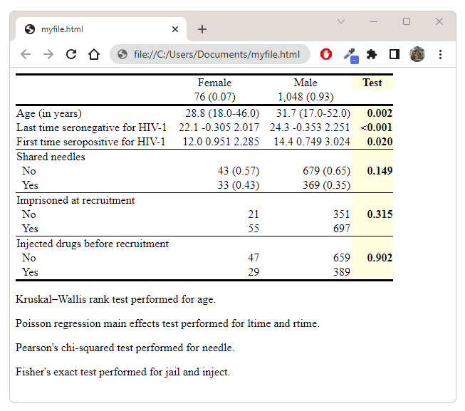
Concerning the additional adjustments, I need to 1) disguise the variable identify male within the desk header and alter the group labels No and Sure to Feminine and Male, respectively, 2) add horizontal traces between steady variables and categorical variables and in addition between totally different categorical variables, 3) daring the p-values for the assessments and spotlight the check column with a light-yellow shade, and 4) add custom-made notes to the desk exhibiting the check varieties for various variables. Let’s use the next gather instructions to make these adjustments:
. gather model header male, title(disguise)

. gather label ranges male 0 "Feminine", modify

. gather label ranges male 1 "Male", modify

. gather model cell var[rtime 1.needle 1.jail], border( backside, width(1))

. gather model cell male[_dtable_test], shading( background(lightyellow)) font(, daring)

. gather notes "Kruskal–Wallis rank check carried out for age."

. gather notes "Poisson regression primary results check carried out for ltime and rtime."

. gather notes "Pearson's chi-squared check carried out for needle."

. gather notes "Fisher's precise check carried out for jail and inject."

. gather format
Please observe the Stata Outcomes window can present a few of these adjustments, but it surely can’t present modifications such because the shading colour. We are able to open the Tables builder and ensure there that we’ve got the precise desk model that we needed. We are able to open the Tables builder from the menu by clicking on Statistics > Summaries, tables, and assessments > Tables and collections > Construct and magnificence desk.
We are able to see how the desk appears to be like proper now within the preview window within the Tables builder.
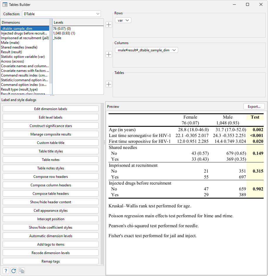
After we export the desk to different paperwork, the exported desk will look the identical as what’s proven right here. Now allow us to export the desk to an .html file.
. gather export myfile.html, substitute
Right here is our ensuing doc:
Generate a full report together with the desk
As a result of dtable creates tables of descriptive statistics, and one of these desk is often included as Desk 1 in technical manuscripts, chances are you’ll need to insert the desk obtained with dtable into a bigger doc as an alternative of solely exporting the desk as a doc. If that’s the case, you should use putdocx gather, putpdf gather, or putexcel ul_cell = gather to export the desk if you’re making a doc utilizing, respectively, putdocx, putpdf, or putexcel. On this method, the desk may be put anyplace within the doc together with different content material. Right here is an instance of utilizing putdocx to create a doc together with the above desk:
webuse idu, clear
putdocx clear
putdocx start
// Add a title
putdocx paragraph, model(Title)
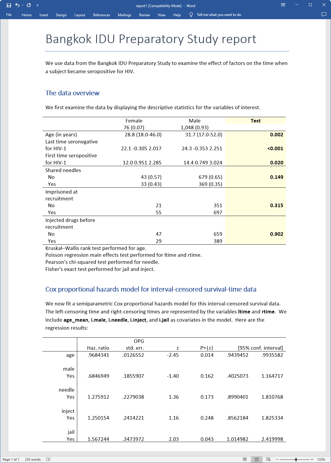
putdocx textual content ("Bangkok IDU Preparatory Examine report")
putdocx textblock start
We use information from the Bangkok IDU Preparatory Examine to look at
the impact of things on the time when a topic grew to become
seropositive for HIV.
putdocx textblock finish
// Add a heading
putdocx paragraph, model(Heading1)
putdocx textual content ("The information overview")
putdocx textblock start
We first look at the information by displaying the descriptive
statistics for the variables of curiosity.
putdocx textblock finish
dtable, by(male, assessments testnotes nototal) ///
pattern(, statistic(frequency proportion) ///
place(seplabels) ) steady(age, statistics(imply minmax) check(kwallis)) ///
steady(ltime rtime, statistics(imply skewness kurtosis) check(poisson)) ///
issue(needle, statistics(fvfrequency fvproportion)) ///
issue(jail inject, statistics(fvfrequency) check(fisher)) ///
outline(minmax = min max, delimiter(-)) nformat(%9.1f imply minmax) ///
sformat("(%s)" fvproportion minmax proportion) ///
nformat(%9.2f proportion fvproportion)
gather model header male, title(disguise)
gather label ranges male 0 "Feminine", modify
gather label ranges male 1 "Male", modify
gather model cell var[rtime 1.needle 1.jail], border( backside, width(1))
gather model cell male[_dtable_test], shading( background(lightyellow)) ///
font(, daring)
gather notes "Kruskal–Wallis rank check carried out for age."
gather notes "Poisson regression primary results check carried out for ltime and rtime."
gather notes "Pearson's chi-squared check carried out for needle."
gather notes "Fisher's precise check carried out for jail and inject."
putdocx gather
putdocx paragraph, model(Heading1)
putdocx textual content ("Cox proportional hazards mannequin for interval-censored survival-time information")
putdocx textblock start
We now match a semiparametric Cox proportional hazards mannequin for this
interval-censored survival information. The left-censoring time and
right-censoring occasions are represented by the variables
<> and
<>. We embody
<>, <>,
<>, <>,
and <> as covariates within the mannequin.
Listed here are the regression outcomes:
putdocx textblock finish
stintcox age i.male i.needle i.inject i.jail, interval(ltime rtime)
putdocx desk outcomes = etable
putdocx save report1, substitute
Utilizing the above code, we create the file report1.docx, which appears to be like like
This report can be reproducible. Rerun your instructions at any time and re-create your report. You possibly can see https://www.stata.com/options/overview/truly-reproducible-reporting/ for extra data concerning reproducible studies.
Abstract
On this weblog put up, I’ve proven you among the options and enjoyable issues you are able to do utilizing dtable in Stata 18. It has so many options that I can’t present them multi function put up. Now chances are you’ll be able to open your Stata and check out dtable your self. I hope I’ve offered you with some helpful demonstrations, and which will offer you a superb begin.
To learn extra about dtable, please go to
You can too watch the next video tutorial on our YouTube channel:
Reference
Zeng, D., L. Mao, and D. Lin. 2016. Most probability estimation for semiparametric transformation fashions with interval-censored information. Biometrika 103: 253–271. https://doi.org/10.1093/biomet/asw013