This weblog put up focuses on new options and enhancements. For a complete checklist, together with bug fixes, please see the launch notes.
LLM inference at scale sometimes includes deploying a number of replicas of the identical mannequin behind a load balancer. The usual strategy treats these replicas as interchangeable and routes requests randomly or round-robin throughout them.
However LLM inference is not stateless. Every duplicate builds up a KV cache of beforehand computed consideration states. When a request lands on a reproduction with out the related context already cached, the mannequin has to recompute all the things from scratch. This wastes GPU cycles and will increase latency.
The issue turns into seen in three frequent patterns: shared system prompts (each app has one), RAG pipelines (customers question the identical data base), and multi-turn conversations (follow-up messages share context). In all three instances, a naive load balancer forces replicas to independently compute the identical prefixes, multiplying redundant work by your duplicate rely.
Clarifai 12.3 introduces KV Cache-Conscious Routing, which routinely detects immediate overlap throughout requests and routes them to the duplicate most probably to have already got the related context cached. This delivers measurably larger throughput and decrease time-to-first-token with zero configuration required.
This launch additionally consists of Heat Node Swimming pools for sooner scaling and failover, Session-Conscious Routing to maintain consumer requests on the identical duplicate, Prediction Caching for equivalent inputs, and Clarifai Expertise for AI coding assistants.
KV Cache-Conscious Routing
Whenever you deploy an LLM with a number of replicas, commonplace load balancing distributes requests evenly throughout all replicas. This works effectively for stateless purposes, however LLM inference has state: the KV cache.
The KV cache shops beforehand computed key-value pairs from the eye mechanism. When a brand new request shares context with a earlier request, the mannequin can reuse these cached computations as a substitute of recalculating them. This makes inference sooner and extra environment friendly.
But when your load balancer would not account for cache state, requests get scattered randomly throughout replicas. Every duplicate finally ends up recomputing the identical context independently, losing GPU sources.
Three Frequent Patterns The place This Issues
Shared system prompts are the clearest instance. Each utility has a system instruction that prefixes consumer messages. When 100 customers hit the identical mannequin, a random load balancer scatters them throughout replicas, forcing every one to independently compute the identical system immediate prefix. When you’ve got 5 replicas, you are computing that system immediate 5 instances as a substitute of as soon as.
RAG pipelines amplify the issue. Customers querying the identical data base get near-identical retrieved-document prefixes injected into their prompts. With out cache-aware routing, this shared context is recomputed on each duplicate as a substitute of being reused. The overlap will be substantial, particularly when a number of customers ask associated questions inside a short while window.
Multi-turn conversations create implicit cache dependencies. Comply with-up messages in a dialog share your entire prior context. If the second message lands on a distinct duplicate than the primary, the total dialog historical past needs to be reprocessed. This will get worse as conversations develop longer.
How Compute Orchestration Solves It
Clarifai Compute Orchestration analyzes incoming requests, detects immediate overlap, and routes them to the duplicate most probably to have already got the related KV cache loaded.
The routing layer identifies shared prefixes and directs site visitors to replicas the place that context is already heat. This occurs transparently on the platform degree. You do not configure cache keys, handle periods, or modify your utility code.
The result’s measurably larger throughput and decrease time-to-first-token. GPU utilization improves as a result of replicas spend much less time on redundant computation. Customers see sooner responses as a result of requests hit replicas which might be already warmed up with the related context.
This optimization is on the market routinely on any multi-replica deployment of vLLM or SGLang-backed fashions. No configuration required. No code adjustments wanted.
Heat Node Swimming pools
GPU chilly begins occur when deployments have to scale past their present capability. The standard sequence: provision a cloud node (1-5 minutes), pull the container picture, obtain mannequin weights, load into GPU reminiscence, then serve the primary request.
Setting min_replicas ≥ 1 retains baseline capability at all times heat. However when site visitors exceeds that baseline or failover occurs to a secondary nodepool, you continue to face infrastructure provisioning delays.
Heat Node Swimming pools hold GPU infrastructure pre-warmed and able to settle for workloads.
How It Works
Well-liked GPU occasion sorts have nodes standing by, prepared to simply accept workloads with out ready for cloud supplier provisioning. When your deployment must scale up, the node is already there.
When your main nodepool approaches capability, Clarifai routinely begins making ready the subsequent precedence nodepool earlier than site visitors spills over. By the point overflow occurs, the infrastructure is prepared.
Heat capability is held utilizing light-weight placeholder workloads which might be immediately evicted when an actual mannequin wants the GPU. Your mannequin will get the sources instantly with out competing for scheduling.
This eliminates the infrastructure provisioning step (1-5 minutes). Container picture pull and mannequin weight loading nonetheless occur when a brand new duplicate begins, however mixed with Clarifai’s pre-built base photographs and optimized mannequin loading, scaling delays are considerably diminished.
Session-Conscious Routing and Prediction Caching
Past KV cache affinity, Clarifai 12.3 consists of two further routing optimizations that work collectively to enhance efficiency.
Session-Conscious Routing retains consumer requests on the identical duplicate all through a session. That is notably helpful for conversational purposes the place follow-up messages from the identical consumer share context. As a substitute of counting on KV cache affinity to detect overlap, session-aware routing ensures continuity by routing based mostly on consumer or session identifiers.
This works with none client-side adjustments. The platform handles session monitoring routinely and ensures that requests with the identical session ID land on the identical duplicate, preserving KV cache locality.
Prediction Caching shops outcomes for equivalent enter, mannequin, and model mixtures. When the very same request arrives, the cached result’s returned instantly with out invoking the mannequin.
That is helpful for eventualities the place a number of customers submit equivalent queries. For instance, in a buyer help utility the place customers ceaselessly ask the identical questions, prediction caching eliminates redundant inference calls fully.
Each options are enabled routinely. You do not configure cache insurance policies or handle session state. The routing layer handles this transparently.
Clarifai Expertise
We’re releasing Clarifai Expertise that flip AI coding assistants like Claude Code into Clarifai platform specialists. As a substitute of explaining APIs from scratch, you describe what you need in plain language and your assistant finds the fitting talent and will get to work.
Constructed on the open Agent Expertise commonplace, Clarifai Expertise work throughout 30+ agent platforms together with Claude Code, Cursor, GitHub Copilot, and Gemini. Every talent consists of detailed reference documentation and dealing code examples.
Accessible abilities cowl the total platform: CLI instructions (clarifai-cli), mannequin deployment (clarifai-model-upload), inference (clarifai-inference), MCP server growth (clarifai-mcp), deployment lifecycle administration (clarifai-deployment-lifecycle), observability (clarifai-observability), and extra.
Set up is simple:
As soon as put in, abilities activate routinely when your request matches their description. Ask naturally (“Deploy Qwen3-0.6B with vLLM”) and your assistant generates the right code utilizing Clarifai’s APIs and conventions.
Full documentation, set up directions, and examples right here.
Extra Modifications
Python SDK Updates
Mannequin Serving and Deployment
The clarifai mannequin deploy command now consists of multi-cloud GPU discovery and a zero-prompt deployment circulation. Simplified config.yaml construction for mannequin initialization makes it simpler to get began.
clarifai mannequin serve now reuses present sources when obtainable as a substitute of making new ones. Served fashions are non-public by default. Added --keep flag to protect the construct listing after serving, helpful for debugging and inspecting construct artifacts.
Native Runner is now public by default. Fashions launched through the native runner are publicly accessible with out manually setting visibility.
Mannequin Runner
Added VLLMOpenAIModelClass mother or father class with built-in cancellation help and well being probes for vLLM-backed fashions.
Optimized mannequin runner reminiscence and latency. Diminished reminiscence footprint and improved response latency within the mannequin runner. Streamlined overhead in SSE (Server-Despatched Occasions) streaming.
Auto-detect and clamp max_tokens. The runner now routinely detects the backend’s max_seq_len and clamps max_tokens to that worth, stopping out-of-range errors.
Bug Fixes
Mounted reasoning mannequin token monitoring and streaming in agentic class. Token monitoring for reasoning fashions now accurately accounts for reasoning tokens. Mounted event-loop security, streaming, and gear name passthrough within the agentic class.
Mounted consumer/app context conflicts in CLI. Resolved conflicts between user_id and app_id when utilizing named contexts in CLI instructions.
Mounted clarifai mannequin init listing dealing with. The command now accurately updates an present mannequin listing as a substitute of making a subdirectory.
Able to Begin Constructing?
KV Cache-Conscious Routing is on the market now on all multi-replica deployments. Deploy a mannequin with a number of replicas and routing optimizations are enabled routinely. No configuration required.
Set up Clarifai Expertise to show Claude Code, Cursor, or any AI coding assistant right into a Clarifai platform professional. Learn the full set up information and see the entire launch notes for all updates in 12.3.
Enroll to begin deploying fashions with clever request routing, or be part of the neighborhood on Discord right here when you’ve got any questions.
From the chilly snap this winter to the US struggle with Iran, rising vitality payments are making headlines. However there’s a bigger story behind spikes in gas-utility prices, one many years within the making.
The primary driver of those payments was once the worth of gasoline itself. Now it’s the gasoline system infrastructure, like pipeline replacements: That accounted for about 70 p.c of buyer payments in 2024, whereas gasoline was simply 30 p.c.
“The sleeper perpetrator of those constantly rising payments is, actually, the infrastructure,” stated Kristin Bagdanov, co-author of a brand new report by the Constructing Decarbonization Coalition (BDC) that was revealed Tuesday.
Electrical payments have been on the rise too, however not almost on the similar charge as these for gasoline. In 2025, gasoline utility payments rose 60 p.c sooner than electrical ones and 4 occasions sooner than inflation, the report discovered. All of this comes as gasoline use declines, a results of extra environment friendly gasoline boilers alongside a push in direction of electrification as states work to fulfill local weather targets.
The spike in the price of gasoline itself is the cherry on high of a system that has grown more and more costly through the years. Within the final decade, gasoline utility spending on pipes and supply tripled, reaching $28 billion in 2023, the report notes. Utilities started changing their pipelines extra quickly in 2010 — partially due to the lifespan of pipes, which is able to ultimately corrode and leak.
Gasoline crews work on repairing a ruptured pure gasoline line on December 30, 2025, in Castaic, California.Kayla Bartkowski/Los Angeles Occasions through Getty Photographs
Between then and 2014, 27 states applied insurance policies that allowed utilities to recuperate these prices extra rapidly, elevating charges for purchasers. In complete, not less than 42 states have enacted some type of rider, surcharge or program to speed up the substitute of gasoline distribution pipelines, in keeping with information from the American Gasoline Affiliation, a utility commerce group.
Utility spending has far outpaced progress within the gasoline buyer base, which is up simply 8.5 p.c in complete since 2000, the BDC report says, citing information from the US Power Info Administration. In the meantime, residential gasoline demand has remained almost flat for the reason that Nineteen Seventies.
“Meaning persons are paying extra per pipe than they’d been 30 years in the past,” Bagdanov stated, making a gasoline system that’s “underutilized and dearer.”
If utilities had continued their pre-2010 tempo of funding, BDC calculates that US clients would have saved an estimated $130 billion in complete by 2023, or $1,723 per family utilizing gasoline. The gas-utility trade, nevertheless, emphasizes value financial savings for residents who use gasoline as a substitute of electrical energy. The American Gasoline Affiliation writes in its 2026 Playbook that “properties that use pure gasoline for heating, cooking and garments drying save a mean of $1,030 per yr in comparison with properties that use electrical energy for those self same purposes.”
The BDC report argues that continued investments within the gasoline system don’t make sense. States with mandated local weather targets must spend money on electrification and dramatically scale back fossil gasoline use. The place replacements are wanted for gasoline pipes which can be previous and unsafe, there are different choices, stated Kevin Carbonnier, co-author of the report, like geothermal vitality networks, demand-response applications to make use of vitality extra effectively, sewer warmth restoration and electrification.
“Let’s have a look at non-pipe alternate options to see if we are able to modernize our properties and our infrastructure, fairly than placing within the hundreds of thousands of {dollars} to exchange that pipe,” he stated.
A rising variety of states have taken that sentiment to coronary heart. Since 2020, utility regulators in 13 states and Washington, DC, have opened proceedings on transitioning away from pure gasoline for heating. Lawmakers are contemplating their choices, too.
In Minnesota, for instance, a brand new proposed invoice would enable gasoline utilities to construct geothermal vitality networks within the state, a transfer that would scale back fossil gasoline use. “We all know that decarbonizing heating and cooling is likely one of the greatest challenges that we’ve within the clear vitality transition,” state Rep. Athena Hollins, sponsor of the invoice, stated at a listening to in late March. The invoice has obtained robust assist from Minnesota’s largest pure gasoline utility, CenterPoint Power, together with labor teams.
Massachusetts is already increasing its first utility-led thermal vitality neighborhood, whereas Maryland regulators are at the moment accepting testimony on their assessment of whether or not state gasoline utilities’ planning is in keeping with the state’s local weather targets.
State insurance policies and incentives are additionally serving to to make electrification instruments, like warmth pumps, extra inexpensive. In California, legislators are contemplating the Warmth Pump Entry Act to make it sooner, simpler, and cheaper to put in warmth pumps for cooling and heating, a part of a push to assist the state attain carbon neutrality by 2045.
In 2025, warmth pumps outsold gasoline furnaces within the U.S. for the fourth yr in a row. Plug-in balcony photo voltaic is receiving mounting curiosity as effectively. “We’re seeing quite a lot of electrification and other people disconnecting from gasoline as they improve their properties to those trendy, sooner, higher, extra snug, environment friendly home equipment,” Carbonnier stated.
Whereas the Trump administration has slashed clear vitality incentives on a federal stage, “what we see on the state stage is definitely like quite a lot of sturdy progress,” Bagdanov stated. “It simply reinforces the truth that as that gasoline system continues to get increasingly costly, these clean-heat options get even higher and extra inexpensive.”
1000’s of fans, professionals and curious skywatchers will collect this weekend for the world’s largest and most spectacular astronomy and area expo.
The Northeast Astronomy Discussion board & Area Expo 2026 (NEAF) takes place April 11–12 at Rockland Group School in Suffern, New York, and marks the occasion’s thirty fifth 12 months. The 2-day occasion options area talks with NASA specialists, cutting-edge tech and hands-on stargazing experiences.
Over time, NEAF has grown into “the world famend discussion board of area and astronomy pursuits” and “the preeminent symposium for award successful talks, workshops, courses and conferences,” drawing greater than 4,000 professionals, amateurs and area fans yearly, all coming collectively to share pursuits and passions, NEAF producer Ed Siemenn informed Area.com.
Greater than 100 distributors and exhibitors from around the globe attend NEAF, representing main producers and sellers. That breadth, Siemenn famous, makes it “one of many largest commerce exhibits and collaborative venues of its form on this planet” in addition to “an fanatic’s purchasing paradise.”
“NEAF is a real ‘Discussion board’ of occasions for anybody who has gazed upward to the evening sky and located a curiosity to grasp the cosmos that lies past our personal skinny ambiance,” Siemenn stated. “Annually NEAF searches the globe to current an all star line up of wonderful friends which can be making historical past right this moment. Nowhere else can you discover such an thrilling array of applications introduced collectively in a single place and at one time.”
The exhibit corridor spans telescope makers, imaging gear suppliers, astronomy golf equipment and area organizations, complemented by dwell demonstrations, photo voltaic observing, newbie telescope periods, planetarium programming and a big raffle.
Amongst this 12 months’s standout audio system is Anna Fisher, a trailblazing NASA astronaut and one of many first girls to fly in area. She made historical past in 1984 aboard the area shuttle Discovery on mission STS-51A, serving to to seize and return two malfunctioning satellites — one of the vital technically difficult rescue operations ever carried out in orbit. A doctor in addition to an astronaut, she later turned the first mom to journey to area, and has performed a key function in shaping NASA’s human spaceflight applications by way of a long time of service.
Breaking area information, the newest updates on rocket launches, skywatching occasions and extra!
Becoming a member of her is Pettit, a veteran NASA astronaut identified for his long-duration missions aboard the Worldwide Area Station and his method to science in microgravity. Pettit has spent greater than a 12 months in area throughout a number of missions, conducting experiments starting from fluid physics to orbital images, whereas additionally gaining a following for his putting photographs of Earth and the cosmos taken from orbit. His work blends engineering, science and creativity, providing a singular perspective on life and analysis in area.
Different notable audio system in this 12 months’s lineup embody veteran astronauts and main area science voices, resembling Robert Gibson (Hoot Gibson), Michelle Thaller, Ken Kremer, David McComas, Mike Ciannilli, Jim Garvin, Gerry Griffin and Kevin Schindler. The occasion might be hosted by NEAF Talks Grasp of Ceremonies Vince Coulehan and Area.com’s personal skywatching columnist Joe Rao, who will assist open the ceremony on Saturday. A full schedule of occasions is offered on-line.
Shows will cowl human spaceflight, astrophysics, mission operations and ongoing exploration efforts, reflecting NEAF’s long-standing give attention to each training and inspiration, based on the occasion program.
Main as much as the primary occasion, the Northeast Astro-Imaging Convention (NEAIC) will run April 9–10, providing workshops and talks devoted to astrophotography methods, processing workflows and superior imaging instruments for newbies and skilled imagers alike.
Tickets can be found prematurely on-line or on the door, with free admission for youngsters and school college students with legitimate ID. One-day passes begin at $41, or $75 for each days when bought on-line, with increased costs on the door.
“Fairly merely — if area and astronomy curiosity you, then you definately don’t wish to miss NEAF,” Siemenn stated.
Amazon Bedrock repeatedly releases new basis mannequin (FM) variations with higher capabilities, accuracy, and security. Understanding the mannequin lifecycle is crucial for efficient planning and administration of AI purposes constructed on Amazon Bedrock. Earlier than migrating your purposes, you’ll be able to check these fashions by means of the Amazon Bedrock console or API to judge their efficiency and compatibility.
This submit reveals you the best way to handle FM transitions in Amazon Bedrock, so you can also make certain your AI purposes stay operational as fashions evolve. We focus on the three lifecycle states, the best way to plan migrations with the brand new prolonged entry function, and sensible methods to transition your purposes to newer fashions with out disruption.
Amazon Bedrock mannequin lifecycle overview
A mannequin supplied on Amazon Bedrock can exist in one in all three states: Lively, Legacy, or Finish-of-Life (EOL). Their present standing is seen each on the Amazon Bedrock console and in API responses. For instance, once you make a GetFoundationModel or ListFoundationModels name, the state of the mannequin shall be proven within the modelLifecycle area within the response.
The next diagram illustrates the main points round every mannequin state.
The state particulars are as follows:
ACTIVE – Lively fashions obtain ongoing upkeep, updates, and bug fixes from their suppliers. Whereas a mannequin is Lively, you need to use it for inference by means of APIs like InvokeModel or Converse, customise it (if supported), and request quota will increase by means of AWS Service Quotas.
LEGACY – When a mannequin supplier transitions a mannequin to Legacy state, Amazon Bedrock will notify clients with at the very least 6 months’ advance discover earlier than the EOL date, offering important time to plan and execute a migration to newer or different mannequin variations. Through the Legacy interval, current clients can proceed utilizing the mannequin, although new clients is likely to be unable to entry it, and current clients may lose entry for inactive accounts if they don’t name the mannequin for a interval of 15 days or extra. Organizations ought to be aware that creating new provisioned throughput by mannequin models turns into unavailable, and mannequin customization capabilities may face restrictions. For fashions with EOL dates after February 1, 2026, Amazon Bedrock introduces an extra section throughout the Legacy state:
Public prolonged entry interval – After spending a minimal of three months in Legacy standing, the mannequin enters this prolonged entry section. Lively customers can proceed utilizing it for at the very least one other 3 months till EOL. Throughout prolonged entry, quota improve requests by means of AWS Service Quotas usually are not anticipated to be authorised, so plan your capability wants earlier than a mannequin enters this section. Throughout this era, pricing could also be adjusted (see Pricing throughout prolonged entry under), and clients will obtain notifications in regards to the transition date and any modifications.
END-OF-LIFE (EOL) – When a mannequin reaches its EOL date, it turns into fully inaccessible throughout all AWS Areas except particularly famous within the EOL listing. API requests to EOL fashions will fail, rendering them unavailable to most clients except particular preparations exist between the client and supplier for continued entry. The transition to EOL requires proactive buyer motion—migration doesn’t occur mechanically. Organizations should replace their software code to make use of different fashions earlier than the EOL date arrives. When EOL is reached, the mannequin turns into fully inaccessible for many clients.
After a mannequin launches on Amazon Bedrock, it stays obtainable for at the very least 12 months after launch and stays in Legacy state for at the very least 6 months earlier than EOL. This timeline helps clients plan migrations with out speeding.
Pricing throughout prolonged entry
Through the prolonged entry interval, pricing could also be adjusted by the mannequin supplier. If pricing modifications are deliberate, you can be notified within the preliminary legacy announcement and earlier than any subsequent modifications take impact, so there shall be no shock retroactive value will increase. Clients with current non-public pricing agreements with mannequin suppliers or these utilizing provisioned throughput will proceed to function beneath their present pricing phrases throughout the prolonged entry interval. This makes certain clients who’ve made particular preparations with mannequin suppliers or invested in provisioned capability won’t be unexpectedly affected by any pricing modifications.
Communication Course of for Mannequin State Adjustments
Clients will obtain a notification 6 months previous to a mannequin’s EOL date when the mannequin supplier transitions a mannequin to Legacy state. This proactive communication method ensures that clients have ample time to plan and execute their migration methods earlier than a mannequin turns into EOL.
Notifications embody particulars in regards to the mannequin being deprecated, essential dates, prolonged entry availability, and when the mannequin shall be EOL. AWS makes use of a number of channels to make sure these essential communications attain the appropriate folks, together with:
To be sure to obtain these notifications, confirm and configure your account contact electronic mail addresses. By default, notifications are despatched to your account’s root person electronic mail and alternate contacts (operations, safety, and billing). You possibly can assessment and replace these contacts in your AWS Account web page within the Alternate contacts part. So as to add further recipients or supply channels (reminiscent of Slack or electronic mail distribution lists), go to the AWS Consumer Notifications console and select AWS managed notifications subscriptions to handle your supply channels and account contacts. If you’re not receiving anticipated notifications, test that your electronic mail addresses are accurately configured in these settings and that notification emails from well being@aws.com usually are not being filtered by your electronic mail supplier.
Migration methods and finest practices
When migrating to a more recent mannequin, replace your software code and test that your service quotas can deal with anticipated quantity. Planning forward helps you transition easily with minimal disruption.
Planning your migration timeline
Begin planning as quickly as a mannequin enters Legacy state:
Evaluation section – Consider your present utilization of the legacy mannequin, together with which purposes rely upon it, typical request patterns, and particular behaviors or outputs that your purposes depend on.
Analysis section – Examine the really helpful substitute mannequin, understanding its capabilities, variations from the legacy mannequin, new options that might improve your purposes, and the brand new mannequin’s Regional availability. Overview API modifications and documentation.
Testing section – Conduct thorough testing with the brand new mannequin and examine efficiency metrics between fashions. This helps determine changes wanted in your software code or immediate engineering.
Migration section – Implement modifications utilizing a phased deployment method. Monitor system efficiency throughout transition and keep rollback functionality.
Operational section – After migration, repeatedly monitor your purposes and person suggestions to ensure they’re performing as anticipated with the brand new mannequin.
Technical migration steps
Check your migration completely:
Replace API references – Modify your software code to reference the brand new mannequin ID. For instance, altering from anthropic.claude-3-5-sonnet-20240620-v1:0 to anthropic.claude-sonnet-4-5-20250929-v1:0 or world cross-Area inferenceworld.anthropic.claude-sonnet-4-5-20250929-v1:0. Replace immediate constructions in response to new mannequin’s finest practices. For extra detailed steering, check with Migrate from Anthropic’s Claude Sonnet 3.x to Claude Sonnet 4.x on Amazon Bedrock.
Request quota will increase – Earlier than totally migrating, be sure to have ample quotas for the brand new mannequin by requesting will increase by means of the AWS Service Quotas console if obligatory.
Regulate prompts – Newer fashions may reply in a different way to the identical prompts. Overview and refine your prompts accordingly to the brand new mannequin specs. You too can use instruments such because the immediate optimizer in Amazon Bedrock to help with rewriting your immediate for the goal mannequin.
Replace response dealing with – If the brand new mannequin returns responses in a unique format or with totally different traits, replace your parsing and processing logic accordingly.
Optimize token utilization – Reap the benefits of effectivity enhancements in newer fashions by reviewing and optimizing your token utilization patterns. For instance, fashions that help immediate caching can cut back the associated fee and latency of your invocations.
Testing methods
Thorough testing is essential for a profitable migration:
Facet-by-side comparability – Run the identical requests towards each the legacy and new fashions to check outputs and determine any variations that may have an effect on your software. For manufacturing environments, take into account shadow testing—sending duplicate requests to the brand new mannequin alongside your current mannequin with out affecting end-users. With this method, you’ll be able to consider mannequin efficiency, latency and errors charges, and different operational elements earlier than full migration. Carry out A/B testing for person impression evaluation by routing a managed share of stay visitors to the brand new mannequin whereas monitoring key metrics reminiscent of person engagement, activity completion charges, satisfaction scores, and enterprise KPIs.
Efficiency testing – Measure response occasions, token utilization, and different efficiency metrics to grasp how the brand new mannequin performs in comparison with the legacy model. Validate business-specific success metrics.
Regression and edge case testing – Ensure that current performance continues to work as anticipated with the brand new mannequin. Pay particular consideration to uncommon or complicated inputs that may reveal variations in how the fashions deal with difficult situations.
Conclusion
The mannequin lifecycle coverage in Amazon Bedrock offers you clear phases for managing FM evolution. Transition intervals provide prolonged entry choices, and provisions for fine-tuned fashions show you how to steadiness innovation with stability.
Keep knowledgeable about mannequin states by means of the AWS Well being Dashboard, plan migrations when fashions enter the Legacy state, and check newer variations completely. These tips may help you keep continuity in your AI purposes whereas utilizing improved capabilities in newer fashions.
In case you have additional questions or issues, attain out to your AWS crew. We wish to show you how to and facilitate a clean transition as you proceed to make the most of the newest developments in FM know-how.
For continued studying and implementation help, discover the official AWS Bedrock documentation for complete guides and API references. Moreover, go to the AWS Machine Studying Weblog and AWS Structure Middle for real-world case research, migration finest practices, and reference architectures that may assist optimize your mannequin lifecycle administration technique.
In regards to the authors
Saurabh Trikande is a Senior Product Supervisor for Amazon Bedrock and Amazon SageMaker Inference. He’s keen about working with clients and companions, motivated by the objective of democratizing AI. He focuses on core challenges associated to deploying complicated AI purposes, inference with multi-tenant fashions, price optimizations, and making the deployment of generative AI fashions extra accessible. In his spare time, Saurabh enjoys mountaineering, studying about progressive applied sciences, following TechCrunch, and spending time along with his household.
Melanie Li, PhD, is a Senior Generative AI Specialist Options Architect at AWS based mostly in Sydney, Australia, the place her focus is on working with clients to construct options utilizing state-of-the-art AI/ML instruments. She has been actively concerned in a number of generative AI initiatives throughout APJ, harnessing the facility of LLMs. Previous to becoming a member of AWS, Dr. Li held knowledge science roles within the monetary and retail industries.
Derrick Choo is a Senior Options Architect at AWS who accelerates enterprise digital transformation by means of cloud adoption, AI/ML, and generative AI options. He focuses on full-stack growth and ML, designing end-to-end options spanning frontend interfaces, IoT purposes, knowledge integrations, and ML fashions, with a selected concentrate on laptop imaginative and prescient and multi-modal programs.
Jared Dean is a Principal AI/ML Options Architect at AWS. Jared works with clients throughout industries to develop machine studying purposes that enhance effectivity. He’s inquisitive about all issues AI, know-how, and BBQ.
Julia Bodia is Principal Product Supervisor for Amazon Bedrock.
Pooja Rao is a Senior Program Supervisor at AWS, main quota and capability administration and supporting enterprise growth for the Bedrock Go-To-Market crew. Outdoors of labor, she enjoys studying, touring, and spending time together with her household.
Breakthroughs, discoveries, and DIY ideas despatched six days per week.
In a single nook of a typical 3D printing workshop, failed prints and discarded help constructions pile up like industrial kindling. The know-how is meant to be lean. produce solely what you want, if you want it. However anybody who runs a printer is aware of the truth. Misprints, scaffolding, deserted prototypes: they accumulate.
In a laboratory on the Korea Analysis Institute of Chemical Expertise, a researcher is demonstrating one thing that makes that waste pile appear like a design alternative moderately than an inevitability. He takes a freshly printed object from the printer and crushes it right into a shapeless lump together with his naked fingers. Then he nonchalantly stuffs the lump again into the printer’s materials container. Warmth is utilized. A brand new object emerges from the nozzle, easy and clear. No grinding, no reprocessing into filament. Crush, load, print. That’s it.
The fabric isn’t some unique artificial resin. It’s sulfur—the yellowish industrial byproduct that piles up in literal mountains at oil refineries and pure gasoline crops. Roughly 85 million tons of sulfur pour out of refineries and smelters worldwide yearly. A few of it’s changed into sulfuric acid or fertilizer. However a lot of it simply sits there in yellow mounds on manufacturing facility grounds, ready for a use.
4D printing utilizing sulfur plastic as a uncooked materials. Picture: Korea Analysis Institute of Chemical Expertise
A joint analysis crew led by Dr. Kim Dong-Gyun of the Korea Analysis Institute of Chemical Expertise, Prof. Wie Jeong-Jae of Hanyang College, and Prof. Kim Yong-Seok of Sejong College could have discovered one. Their paper, revealed as a canopy article in Superior Supplies, means that sulfur can resolve the persistent waste drawback that has dogged 3D printing since its inception.
Dr. DongGyun Kim of KRICT, who led the examine, and Jae Hyuk Hwang, a researcher at KRICT and the paper’s first writer Picture: Korea Analysis Institute of Chemical Expertise
Why 3D printing supplies are so laborious to recycle
The issue begins on the molecular degree. Widespread thermoplastics like PLA and ABS can technically be melted down and reused, however each time you reheat them, you’re breaking polymer chains. The fabric will get weaker and fewer elastic. Analysis has proven that recycled plastics can drop under usable efficiency thresholds after as few as three to 5 cycles. And that’s assuming you’re keen to grind down the failed print, soften it at excessive temperatures, and extrude it again into filament of uniform thickness—a course of that’s sluggish, energy-intensive, and infrequently definitely worth the bother for small batches.
Photocurable resins are worse. When UV mild hardens them, it kinds irreversible covalent bonds between the molecules. The ensuing materials gained’t soften. It gained’t dissolve. There isn’t a sensible option to undo the chemistry and get the uncooked materials again.
So the waste drawback in 3D printing is known as a chemistry drawback. As soon as these supplies harden, they’re locked into their closing state. The Korea Analysis Institute crew got down to discover a chemical bond that may be locked and unlocked at will. A cloth that holds its form when wanted and breaks aside on command. They discovered one in sulfur.
A decade of making an attempt to make sulfur helpful
The concept of constructing plastic out of sulfur dates again to 2013, when Jeffrey Pyun’s crew on the College of Arizona produced the primary steady polymer wherein sulfur made up greater than half the fabric. The method, often known as inverse vulcanization, flipped the logic of typical rubber processing. Usually, you add a small quantity of sulfur to harden rubber. Pyun’s crew made sulfur the primary ingredient and added small quantities of natural compounds to carry it collectively.
Sulfur plastic Picture: Korea Analysis Institute of Chemical Expertise
The ensuing materials had uncommon properties. It transmitted infrared mild, making it a candidate for thermal imaging lenses. It may selectively soak up heavy metals like mercury from contaminated water. Over the next decade, labs world wide explored variations on the method.
Nevertheless, adapting sulfur plastic for 3D printing proved stubbornly troublesome. The issue was structural. Contained in the plastic, molecules had been knotted right into a mesh so tight that nothing may transfer by it. That density gave the plastic its power. However it additionally made the fabric too viscous to push by a printer nozzle, even when melted. Researchers tried adjusting sulfur ratios and swapping in several natural crosslinkers, however the basic structure of the community stayed the identical. The mesh was too tight.
Loosening the mesh
Dr. Kim’s crew took a special method. As an alternative of tweaking ingredient ratios inside the current community framework, they redesigned the community itself. They intentionally loosened the crosslinked construction, spacing out the connections between molecular chains.
This was vital as a result of sulfur-sulfur bonds break and reform simply. Warmth breaks them aside. Because it cools they reconnect. Within the outdated, tightly crosslinked constructions, the impact was largely suppressed. The bonds didn’t have sufficient room to rearrange. Within the looser community, these change reactions got here alive. The sensible payoff is a property known as shear-thinning: When compelled by a slim opening, the fabric’s viscosity drops and it flows simply. By means of the printer nozzle it flows like a liquid. As soon as extruded, the bonds reform and the form holds.
Getting the looseness proper was the laborious half. Too free, and the fabric loses its power. With too little crosslinker the sulfur reverts to its elemental kind. It unravels.
“Including too little natural crosslinker makes the fabric overly versatile, and the sulfur finally ends up unraveling again to its unique elemental kind,” Dr. Kim mentioned. “To take care of the specified properties, a sure minimal quantity of crosslinker is required, so we went by a technique of fine-tuning the ratios.”
Objects fabricated utilizing sulfur-plastic-based 4D printing. Picture: Korea Analysis Institute of Chemical Expertise
Crush, load, print once more
What makes this materials genuinely completely different from typical 3D printing plastics is what occurs after printing. As a result of the sulfur-sulfur bonds are reversible, a completed print will be heated again right into a smooth, deformable state at any time. When it cools, the bonds reconnect and the fabric re-solidifies. The form adjustments; the fabric doesn’t degrade. You may take a failed print or a construction that’s outlived its usefulness, crush it, stuff it again into the printer’s hopper, and print one thing new. No grinding. No filament reprocessing. The crew confirmed that materials properties remained steady by as much as ten recycling cycles with out important degradation.
They known as the method ‘closed-loop printing’. Sulfur that was as soon as refinery waste turns into a printable plastic, will get formed right into a helpful construction, and when that construction is not wanted, will get melted down and printed into one thing else. At no level does the fabric depart the cycle as waste.
Printing robots with out motors
Recyclability turned out to be solely the start. The identical dynamic bonds that make the fabric reusable additionally make it responsive. When uncovered to warmth or mild, the bonds break and reform in ways in which enable a printed construction to vary form and transfer based on a pre-designed sample—a functionality often known as 4D printing, the place objects proceed to rework after they depart the printer.
By adjusting the sulfur content material, the crew may tune the temperature at which this shape-memory impact kicks in. At 46 p.c sulfur, the fabric returns to its programmed form at round 14°C. At 63 p.c, the set off temperature rises to about 35°C. At 76 p.c, it’s roughly 52°C. Sure compositions additionally reply to near-infrared mild. And when iron powder is blended in, the fabric turns into magnetically responsive. Temperature, mild, magnetic fields—completely different stimuli will be mixed inside a single printed object.
A 4D-printed object blended with iron particles autonomously opening its lid and releasing its contents in response to a shifting magnet. Picture: Korea Analysis Institute of Chemical Expertise
To show what this implies in observe, the crew printed a number of smooth robots. None of them comprise batteries, wires, or motors. They transfer fully by the fabric’s personal shape-memory response to exterior stimuli.
One was a thread-shaped underwater robotic, only one millimeter thick, that rolled by water in response to magnetic fields. Robotic cleared obstacles practically 1.75 occasions its personal physique thickness. One other was a gripper robotic that opened and closed its arms in response to ambient temperature adjustments. It may decide up and relocate small objects.
Probably the most hanging demonstration was a capsule-shaped robotic designed to hold out a chemical response autonomously. The crew loaded a catalyst inside a 3D-printed sulfur-plastic capsule and sealed it. When the capsule was dropped into an natural solvent answer and the temperature reached 50°C, the lid popped open by itself, releasing the catalyst. Concurrently, a magnet rotating beneath the container spun the capsule like a magnetic stir bar, mixing the answer evenly. After about 60 minutes, the response was full. With out anybody having so as to add the catalyst by hand or stir the answer.
What’s nonetheless lacking
Commercialization is a good distance off. The ten-cycle recycling determine is encouraging, however the crew hasn’t but run long-term checks past a number of dozen cycles. Extra iron powder improves the magnetic response, however above 20 p.c it clogs the nozzle. And no sulfur polymer materials of any form has but reached industrial manufacturing.
“To maneuver past lab-scale outcomes and switch this into precise merchandise, we have to goal particular utility areas and work with corporations from the early levels,” Dr. Kim mentioned.
A single materials, many features
“In the event you take a look at every aspect in isolation, there was prior analysis,” Dr. Kim mentioned. “As an illustration, research utilizing magnetic particles to construct smooth robots, or work demonstrating shape-memory properties with sulfur polymers—these particular person element applied sciences already existed. However that is the primary time all of those have been built-in right into a single materials that may ship so many various features directly.”
That integration is the actual contribution. It’s a materials produced from industrial waste. It’s printable and absolutely recyclable. It will also be programmed to maneuver, reply to its setting, and perform duties by itself. Every of these capabilities existed individually. Placing them collectively in a single printable, crushable, re-printable substance is new.
2025 PopSci Better of What’s New
The 50 most necessary improvements of the 12 months
Most free programs present surface-level principle and a certificates that’s usually forgotten inside every week. Luckily, Google and Kaggle have collaborated to supply a extra substantive different. Their intensive 5 day generative AI (GenAI) course covers foundational fashions, embeddings, AI brokers, domain-specific giant language fashions (LLMs), and machine studying operations (MLOps) by way of every week of whitepapers, hands-on code labs, and stay skilled periods.
The second iteration of this program attracted over 280,000 signups and set a Guinness World File for the most important digital AI convention in a single week. All course supplies at the moment are out there as a self-paced Kaggle Be taught Information, fully freed from cost. This text explores the curriculum and why it’s a worthwhile useful resource for knowledge professionals.
Sensible code labs run immediately on Kaggle notebooks, permitting college students to use ideas instantly. The unique stay model featured YouTube livestreams with skilled Q&A periods and a Discord neighborhood of over 160,000 learners. By acquiring conceptual depth from whitepapers and instantly making use of these ideas in code labs utilizing the Gemini API, LangGraph, and Vertex AI, the course maintains a gradual momentum between principle and apply.
// Day 1: Exploring Foundational Fashions and Immediate Engineering
The course begins with the important constructing blocks. You’ll study the evolution of LLMs — from the unique Transformer structure to trendy fine-tuning and inference acceleration methods. The immediate engineering part covers sensible strategies for guiding mannequin conduct successfully, transferring past fundamental tutorial ideas.
The related code lab entails working immediately with the Gemini API to check varied immediate methods in Python. For many who have used LLMs however by no means explored the mechanics of temperature settings or few-shot immediate structuring, this part rapidly addresses these information gaps.
// Day 2: Implementing Embeddings and Vector Databases
The second day focuses on embeddings, transitioning from summary ideas to sensible purposes. You’ll be taught the geometric methods used for classifying and evaluating textual knowledge. The course then introduces vector shops and databases — the infrastructure crucial for semantic search and retrieval-augmented technology (RAG) at scale.
The hands-on portion entails constructing a RAG question-answering system. This session demonstrates how organizations floor LLM outputs in factual knowledge to mitigate hallucinations, offering a purposeful have a look at how embeddings combine right into a manufacturing pipeline.
// Day 3: Growing Generative Synthetic Intelligence Brokers
Day 3 addresses AI brokers — methods that stretch past easy prompt-response cycles by connecting LLMs to exterior instruments, databases, and real-world workflows. You’ll be taught the core parts of an agent, the iterative improvement course of, and the sensible software of operate calling.
The code labs contain interacting with a database by way of operate calling and constructing an agentic ordering system utilizing LangGraph. As agentic workflows turn into the usual for manufacturing AI, this part gives the required technical basis for wiring these methods collectively.
// Day 4: Analyzing Area-Particular Massive Language Fashions
This part focuses on specialised fashions tailored for particular industries. You’ll discover examples reminiscent of Google’s SecLM for cybersecurity and Med-PaLM for healthcare, together with particulars concerning affected person knowledge utilization and safeguards. Whereas general-purpose fashions are highly effective, fine-tuning for a selected area is usually crucial when excessive accuracy and specificity are required.
The sensible workout routines embody grounding fashions with Google Search knowledge and fine-tuning a Gemini mannequin for a customized job. This lab is especially helpful because it demonstrates the way to adapt a basis mannequin utilizing labeled knowledge — a talent that’s more and more related as organizations transfer towards bespoke AI options.
// Day 5: Mastering Machine Studying Operations for Generative Synthetic Intelligence
The ultimate day covers the deployment and upkeep of GenAI in manufacturing environments. You’ll be taught how conventional MLOps practices are tailored for GenAI workloads. The course additionally demonstrates Vertex AI instruments for managing basis fashions and purposes at scale.
Whereas there isn’t a interactive code lab on the ultimate day, the course gives a radical code walkthrough and a stay demo of Google Cloud’s GenAI assets. This gives important context for anybody planning to maneuver fashions from a improvement pocket book to a manufacturing surroundings for actual customers.
# Splendid Viewers
For knowledge scientists, machine studying engineers, or builders looking for to specialise in GenAI, this course provides a uncommon stability of rigor and accessibility. The multi-format strategy permits learners to regulate the depth primarily based on their expertise degree. Inexperienced persons with a strong basis in Python may also efficiently full the curriculum.
The self-paced Kaggle Be taught Information format permits for versatile scheduling, whether or not you favor to finish it over every week or in a single weekend. As a result of the notebooks run on Kaggle, no native surroundings setup is required; a phone-verified Kaggle account is all that’s wanted to start.
# Remaining Ideas
Google and Kaggle have produced a high-quality academic useful resource out there for free of charge. By combining expert-written whitepapers with instant sensible software, the course gives a complete overview of the present GenAI panorama.
The excessive enrollment numbers and business recognition mirror the standard of the fabric. Whether or not your objective is to construct a RAG pipeline or perceive the underlying mechanics of AI brokers, this course delivers the conceptual framework and the code required to succeed.
Nahla Davies is a software program developer and tech author. Earlier than devoting her work full time to technical writing, she managed—amongst different intriguing issues—to function a lead programmer at an Inc. 5,000 experiential branding group whose shoppers embody Samsung, Time Warner, Netflix, and Sony.
Search “finest agentic AI platform,” and also you’ll drown in a sea of vendor comparisons, function matrices, and power catalogs. The actual enemy isn’t choosing the incorrect vendor, although. Constructing your individual AI resolution can kill your ambitions earlier than they even get off the bottom.
In most enterprises, groups are cobbling collectively their very own mix-and-match stack of open-source instruments, cloud providers, and level options. Advertising has its chatbot builder, IT is experimenting with some hyperscaler’s agent framework, and information science is spinning up vector databases on no matter cloud credit they will scrounge up.
That’s shadow AI in a nutshell, with governance gaps that no compliance audit can simply untangle.
Everybody loves speaking about constructing brokers. That’s the straightforward half.
The half no person desires to confess is that almost all of these brokers won’t ever make it out of a demo. Siloed groups don’t have a unified method to run them, govern them, or preserve them from stepping on one another’s toes.
Enterprises don’t want extra pet initiatives. They want a ruled agent workforce: AI that works throughout groups, clouds, and enterprise programs with out falling aside on the slightest disruption.
Key takeaways
Fragmented AI stacks sluggish enterprises down. Device sprawl and shadow AI make brokers brittle, laborious to control, and tough to scale.
Finish-to-end means unifying construct, deploy, and govern. A single management airplane eliminates handoff failures and will get brokers into manufacturing quicker.
The blank-slate downside is actual. Reference architectures, agent templates, and pre-built starter patterns assist groups ship worth shortly as a substitute of rebuilding from zero.
Openness solely works with governance. Supporting any device or mannequin means nothing with out constant safety, lineage, and coverage controls touring with each agent.
Structural partnerships speed up enterprise readiness. Co-engineered integrations with infrastructure and utility suppliers give groups production-grade agentic workflows with out months of guide setup.
Why fragmentation is the actual enemy to enterprise AI
Stroll into any enterprise at present and ask what number of completely different AI instruments are working throughout the group. The trustworthy reply is often, “We don’t know.” That’s not incompetence. It’s the pure results of groups attempting to carry out their jobs as shortly and precisely as doable.
Shadow AI, duplicated efforts, and area of interest level options are all a part of the issue.
This results in two widespread failure modes that kill extra AI initiatives than any vendor choice mistake ever may:
Device sprawl and “LEGO block” architectures: Someplace alongside the way in which, “transport an AI use case” become a scavenger hunt. Groups are stitching collectively 10–14 instruments, like vector shops, orchestrators, log aggregators, and governance band-aids, simply to get a single agent out the door. Every API and integration level is simply one other output away from failure, safety publicity, or a efficiency meltdown. A challenge that ought to take weeks dissolves right into a multi-month integration saga no person signed up for.
Siloed, cloud-specific stacks that don’t interoperate: Pace over flexibility is how most groups find yourself locked right into a hyperscaler ecosystem. It’s easy crusing till you attempt to plug right into a system you don’t management, deploy in a regulated setting, or collaborate with a accomplice on a unique platform. Then you find yourself selecting between two painful paths: transfer quick and lose management, or preserve management and fall behind.
Any severe dialog about agentic AI platforms has to begin with eliminating this fragmentation. All the pieces else is secondary.
What “end-to-end” truly means for agentic AI
“Finish-to-end” will get thrown round by almost each vendor within the area. However in an enterprise context, it has a particular which means that almost all device collections fail to satisfy.
Actual end-to-end protection spans three crucial phases, every with particular necessities that fragmented device chains wrestle to deal with:
Construct: Groups shouldn’t begin from scratch each time they want an agent. Meaning reference architectures, reusable patterns, and starter kits aligned with actual enterprise workflows.
Function: Single brokers are proofs of idea. Manufacturing programs want dozens or a whole lot of brokers coordinating throughout programs, sharing reminiscence, dealing with errors gracefully, and optimizing for price and latency. That requires refined orchestration, steady analysis, and the flexibility to regulate conduct based mostly on real-world efficiency.
Govern: Lineage, entry management, coverage enforcement, and auditability are wanted the second brokers begin making choices and interacting with actual enterprise programs. Governance isn’t a guidelines. It’s the working system.
Stitching collectively separate instruments for every stage creates drift, governance gaps, and prolonged time-to-production. Groups spend extra time on integration than innovation, and by the point they’re able to deploy, the enterprise necessities have already moved on.
From constructing brokers to working an agent workforce
Most platform conversations go off the rails by specializing in constructing particular person brokers as a substitute of working a workforce of brokers at scale.
That shift adjustments every thing. Operating a workforce means you want:
Shared reminiscence so brokers can be taught from one another’s interactions
Constant reasoning conduct so brokers don’t make contradictory choices
Centralized insurance policies that replace throughout your complete workforce with out redeploying every thing
Unified observability so you may debug multi-agent workflows with out chasing logs throughout a dozen completely different programs
Most significantly, you want agent lifecycle administration on the workforce degree. New brokers ought to mechanically inherit organizational data and insurance policies. Updates ought to roll out constantly throughout associated brokers to forestall coordination failures.
Constructing particular person brokers is a growth downside. Operating an agent workforce is an operational problem that requires platform-level pondering. The 2 require basically completely different approaches.
remedy the clean slate downside
The {industry} loves to supply infinite flexibility, as if giving groups a clean canvas is a present. It isn’t. With out a place to begin, groups spend months making foundational choices which have already been solved elsewhere, time-to-value slipping straight into the following fiscal yr.
What groups really want is momentum.
Meaning beginning with absolutely fashioned agent templates and reference architectures formed round actual enterprise workflows. Not hypotheticals or tutorial examples, however actual doc pipelines, provide chain brokers, and customer support automations with the laborious edge circumstances already accounted for.
The most effective templates aren’t code samples polished for a convention demo. They’re production-ready patterns co-engineered with the infrastructure and utility suppliers enterprises already run on, masking safety, governance, error dealing with, and integrations from the beginning.
The distinction in final result is critical. Groups that begin from confirmed patterns ship in weeks. Groups that begin from scratch are nonetheless constructing foundations when the enterprise necessities change.
When the query turns into “What has AI truly delivered?”, clean slates gained’t have a solution. Confirmed patterns will.
Why a unified, vendor-neutral management airplane issues
Enterprise AI groups face a structural pressure: the instruments and infrastructure they should transfer quick are hardly ever the identical ones IT wants to keep up management, safety, and compliance.
That pressure doesn’t resolve itself. It must be designed round.
A unified management airplane provides each group — AI builders, IT, safety, and enterprise house owners — a single working setting, with out forcing them to desert the instruments they already use. Fashions, databases, frameworks, and deployment targets stay versatile. Governance, lineage, and coverage enforcement journey with each agent, no matter the place it runs.
This issues most on the edges: sovereign cloud deployments, regulated industries, air-gapped environments, and hybrid infrastructure. These are exactly the conditions the place tool-by-tool governance breaks down, and the place a single management airplane proves its worth.
Vendor neutrality isn’t a function. It’s the prerequisite for enterprise AI that may scale past a single group, a single cloud, or a single use case. As AI turns into extra deeply embedded in enterprise programs, the flexibility to control throughout any setting turns into the one sustainable path ahead.
What deep infrastructure partnerships truly allow
Not all know-how partnerships are equal. Emblem-level integrations add a reputation to a slide. Structural, co-engineered partnerships form platform structure and alter what’s truly doable for enterprise groups.
The sensible distinction reveals up in time and complexity. When infrastructure capabilities like inference microservices, reasoning fashions, guardrail frameworks, GPU optimizations, and choice engines are co-engineered right into a platform somewhat than bolted on, groups get entry to them with out months of guide setup, validation, and tuning.
That acceleration unlocks use circumstances that require combining reasoning, simulation, and optimization collectively:
Provide chain routing that considers real-time constraints and optimizes throughout a number of goals
Digital twinsthat simulate complicated eventualities and advocate actions
Scientific workflows that purpose via affected person information whereas sustaining strict privateness controls
Operational reliability issues as a lot as technical depth. Manufacturing-grade architectures have to be validated throughout cloud, on-premises, sovereign, and air-gapped environments. Co-engineered integrations carry that validation with them. Groups inherit it somewhat than having to construct it themselves.
The technical and organizational affect of unifying construct, deploy, and govern
The technical case for unifying construct, deploy, and govern is properly understood. The organizational affect is the place the actual breakthroughs occur.
Assumptions keep intact via each handoff. The complete multi-agent workflow is traceable in a single place, so when one thing misbehaves, groups can diagnose and repair it with out searching via scattered logs throughout disconnected programs.
Organizationally, a unified platform creates shared readability. AI groups, IT, safety, compliance, and enterprise house owners function from the identical supply of reality. Governance stops being a bureaucratic burden handed between groups and turns into a shared working language constructed into the platform itself.
That shift has a direct impact on shadow AI. When the official platform is less complicated to make use of than rogue alternate options, groups cease constructing round it. Fragmentation recedes, not as a result of it was mandated away, however as a result of the higher path grew to become apparent.
What multi-agent orchestration truly requires
Single-agent demos make AI look easy. Multi-agent programs reveal the actual complexity.
The second you progress past one agent, the gaps in most toolchains turn out to be apparent. Shared reminiscence, constant governance, workflow supervision, and unified debugging aren’t elective options. They’re the inspiration that retains multi-agent programs from turning into unmanageable.
Efficient multi-agent orchestration requires a number of capabilities working collectively: dependency administration and retries to deal with failures gracefully, dynamic workload optimization to steadiness price and efficiency throughout brokers, and constant security and reasoning guardrails utilized uniformly throughout your complete system.
With out these, multi-agent workflows create extra operational threat than they eradicate. With them, a coordinated agent workforce turns into doable: one the place brokers share context, function below constant insurance policies, and escalate appropriately after they attain the boundaries of their autonomy.
The workforce analogy holds right here. A functioning workforce, human or AI, wants coordination, shared data, guardrails, and clear escalation paths. Orchestration is what makes that doable at scale.
What a unified platform truly delivers
In some unspecified time in the future, the structure dialogue has to present method to outcomes. Right here’s what enterprises constantly see when the AI lifecycle is correctly unified:
Manufacturing timelines collapse. Groups that used to spend 12–18 months on construct cycles ship in weeks after they’re not rebuilding foundational infrastructure from scratch. The distinction isn’t effort — it’s beginning place.
Inference prices keep manageable. Multi-agent programs can burn via budgets quicker than they generate insights. Actual-time workload optimization and GPU-aware scheduling preserve efficiency excessive and prices predictable.
Resilience will increase. When orchestration, retries, and error dealing with are dealt with on the platform degree, a single failure can’t topple a complete workflow. Points floor earlier than they turn out to be customer-visible outages.
Governance threat shrinks. Lineage, entry management, and coverage enforcement stay constant throughout all brokers. No blind spots, no thriller programs, no surprises in manufacturing. Audits turn out to be routine somewhat than disruptive.
These outcomes share a standard trigger: When the complete lifecycle is unified, groups spend their vitality on issues that matter to the enterprise as a substitute of issues created by their very own infrastructure.
There’s a degree the place gathering extra instruments stops being a method and begins being a legal responsibility. Each addition creates one other integration to keep up, one other governance hole to shut, and one other level of failure to debug on the worst doable second.
The enterprises making actual progress with agentic AI aren’t those with the longest device lists. They’re those that stopped stitching and began working — with platforms that deal with coordination, governance, and lifecycle administration as core features somewhat than afterthoughts.
An agent workforce must behave like an actual group: coordinated, dependable, scalable, and aligned with enterprise outcomes. That doesn’t occur accidentally. It occurs by design.
Prepared to maneuver from experiments to production-grade affect? See how the Agent Workforce Platform works.
FAQs
What makes an agentic AI platform actually “end-to-end”?
An end-to-end agentic AI platform unifies your complete lifecycle, constructing brokers, orchestrating multi-agent workflows, deploying them throughout environments, and governing them with constant insurance policies. Most distributors provide a group of instruments that should be stitched collectively manually.
A real end-to-end platform supplies a single management airplane with shared lineage, observability, and governance, so groups can transfer from prototype to manufacturing with out rebuilding every thing.
Why is fragmentation such a significant downside for enterprises?
When groups use completely different instruments, LLMs, and workflows, enterprises find yourself with brittle brokers, inconsistent insurance policies, duplicated infrastructure, and safety blind spots. Most manufacturing failures occur on the handoff between AI, IT, and DevOps.
Fragmentation additionally fuels shadow AI, the place groups construct unmanaged brokers with out oversight. A unified platform removes these gaps by giving all stakeholders a shared setting and the governance guardrails they want.
How does DataRobot differ from hyperscalers or open-source toolchains?
Hyperscalers and open-source stacks present parts like vector shops, LLMs, gateways, observability instruments, however clients should assemble, combine, and safe them themselves. DataRobot supplies a single platform that unifies these items, helps any mannequin or framework, and embeds governance from day one.
The distinction is agent lifecycle administration, multi-agent orchestration, and vendor-neutral governance that scales throughout the enterprise.
How does the NVIDIA partnership enhance enterprise readiness?
DataRobot is co-engineered with NVIDIA, giving clients day-zero entry to NVIDIA NIMs, NeMo Guardrails, choice optimizers like cuOpt, and industry-specific SDKs with out guide setup.
These integrations flip superior fashions and infrastructure into usable, production-grade agentic patterns that might in any other case require months of meeting and validation.
Why does governance have to be embedded from the beginning?
Governance added on the finish creates gaps in lineage, safety, entry management, and auditability, particularly when brokers transfer between instruments. DataRobot embeds governance into each stage of the lifecycle: versioning, approvals, coverage enforcement, monitoring, and runtime controls are utilized mechanically. This prevents drift, ensures reproducibility, and offers AI leaders visibility throughout all brokers and workloads, even in extremely regulated environments.
How does DataRobot help multi-agent programs at scale?
Multi-agent programs break simply when orchestrators, instruments, and security frameworks aren’t aligned. DataRobot handles coordination, retries, shared reminiscence, coverage consistency, and debugging throughout brokers via Covalent orchestration, syftr optimization, and NVIDIA guardrails. As an alternative of working remoted agent demos, enterprises can run a ruled, scalable workforce of brokers that collaborate reliably throughout programs.
Google says Gmail end-to-end encryption (E2EE) is now obtainable on all Android and iOS gadgets, permitting enterprise customers to learn and compose emails with out further instruments.
Beginning this week, encrypted messages shall be delivered as common emails to Gmail recipients’ inboxes in the event that they use the Gmail app.
Recipients who haven’t got the Gmail cell app and use different e-mail companies can learn them in an internet browser, whatever the machine and repair they’re utilizing.
“For the primary time, customers can compose and browse these E2EE messages natively throughout the Gmail app on Android and iOS. No must obtain additional apps or use mail portals. Customers with a Gmail E2EE license can ship an encrypted message to any recipient, no matter what e-mail deal with the recipient has,” Google introduced on Thursday.
“This launch combines the best stage of privateness and information encryption with a user-friendly expertise for all customers, enabling easy encrypted e-mail for all clients from small companies to enterprises and public sector.”
This characteristic is now obtainable for all client-side encryption (CSE) customers with Enterprise Plus licenses and the Assured Controls or Assured Controls Plus add-on after admins allow the Android and iOS purchasers within the CSE admin interface through the Admin Console.
To ship an end-to-end encrypted message, Gmail customers must activate the “Further encryption” choice by clicking the Lock icon when writing the message.
Writing E2EE messages and studying them with out the app (Google)
In October, Google additionally introduced that Gmail enterprise customers can now ship end-to-end encrypted emails to recipients on any e-mail service or platform.
Gmail’s end-to-end encryption (E2EE) characteristic is powered by the client-side encryption (CSE) technical management, which permits Google Workspace organizations to make use of encryption keys they management and are saved outdoors Google’s servers to guard delicate paperwork and emails.
This fashion, the messages and attachments are encrypted on the shopper earlier than being despatched to Google’s servers, which helps meet regulatory necessities corresponding to information sovereignty, HIPAA, and export controls by making certain that Google and third events cannot learn any of the info.
Gmail CSE was launched in Gmail on the internet in December 2022 as a beta check, following an preliminary beta rollout to Google Drive, Google Docs, Sheets, Slides, Google Meet, and Google Calendar, and it reached basic availability for Google Workspace Enterprise Plus, Training Plus, and Training Normal clients in February 2023.
The corporate started rolling out its new end-to-end encryption (E2EE) mannequin in beta for Gmail enterprise customers in April 2025.
Automated pentesting proves the trail exists. BAS proves whether or not your controls cease it. Most groups run one with out the opposite.
This whitepaper maps six validation surfaces, exhibits the place protection ends, and gives practitioners with three diagnostic questions for any device analysis.
After a 10-day journey to the far facet of the moon, the astronauts of the Artemis II mission are returning to Earth. However within the phrases of NASA administrator Jared Isaacman, the mission shouldn’t be over till everybody arrives residence safely. The reentry of the Orion capsule issues as a lot because the lunar journey itself: It’s the final take a look at to show that the house company has mastered the expertise wanted to usher in a brand new period of deep house exploration.
Based on NASA’s schedule, Artemis II will reenter Earth’s ambiance on Friday, April 10, at 5:07 pm PDT. The published, as with liftoff, might be accessible for viewing on NASA+ and streaming platforms comparable to Amazon Prime, Apple TV, Netflix, and HBO Max. It’s also possible to watch on NASA’s YouTube livestream beneath.
Broadcast occasions throughout the US:
San Francisco: 5:07 pm
Denver: 6:07 pm
Chicago: 7:07 pm
New York: 8:08 pm
Reentry Particulars
If all goes in accordance with plan, the crewed module will enter the ambiance close to southeast Hawaii at a most pace of 38,400 kmh and can take simply 13 minutes to splash down within the Pacific Ocean off the coast of California.
Throughout entry, the surface of the capsule will attain 2,760 levels Celsius. The crew will expertise as much as 3.9 g’s, which implies they’ll really feel a drive equal to almost 4 occasions their weight after spending per week in microgravity.
individuals! When you’ve got ever wished to know how linear regression works or simply refresh the primary concepts with out leaping between plenty of totally different sources – this text is for you. It’s an additional lengthy learn that took me greater than a 12 months to write down. It’s constructed round 5 key concepts:
Visuals first. It is a comic-style article: studying the textual content helps, however it’s not required. A fast run by means of the pictures and animations can nonetheless provide you with a stable understanding of how issues work. There are 100+ visuals in complete;
Animations the place they could assist (33 complete). Pc science is finest understood in movement, so I exploit animations to clarify key concepts;
Newbie-friendly. I stored the fabric so simple as doable, to make the article straightforward for newbies to comply with.
Reproducible. Most visuals have been generated in Python, and the code is open supply.
Deal with observe. Every subsequent step solves an issue that reveals up within the earlier step, so the entire article stays linked.
Another factor: the put up is simplified on goal, so some wording and examples could also be a bit tough or not completely exact. Please don’t simply take my phrase for it – assume critically and double-check my factors. For crucial components, I present hyperlinks to the supply code so you possibly can confirm all the things your self.
Desk of contents
Who’s this text for
Skip this paragraph, simply scroll by means of the article for 2 minutes and take a look at the visuals. You’ll instantly know if you wish to learn it correctly (the primary concepts are proven within the plots and animations). This put up is for newbies and for anybody working with knowledge – and in addition for knowledgeable individuals who need a fast refresh.
What this put up covers
The article is structured in three acts:
Linear regression: what it’s, why we use it, and the best way to match a mannequin;
Learn how to consider the mannequin’s efficiency;
Learn how to enhance the mannequin when the outcomes are usually not adequate.
At a excessive stage, this text covers:
data-driven modeling;
analytical answer for linear regression, and why it’s not all the time sensible;
methods to judge mannequin high quality, each visually and with metrics;
A number of linear regression, the place predictions are based mostly on many options;
the probabilistic aspect of linear regression, since predictions are usually not actual and it is very important quantify uncertainty;
methods to enhance mannequin high quality, from including complexity to simplifying the mannequin with regularization.
Extra particularly, it walks by means of:
the least squares technique for easy linear regression;
regression metrics reminiscent of R², RMSE, MAE, MAPE, SMAPE, together with the Pearson correlation coefficient and the coefficient of willpower, plus visible diagnostics like residual plots;
most probability and prediction intervals;
practice/take a look at splits, why they matter and the best way to do them;
outlier dealing with strategies, together with RANSAC, Mahalanobis distance, Native Outlier Issue (LOF), and Cook dinner’s distance;
knowledge preprocessing, together with normalization, standardization, and categorical encoding;
the linear algebra behind least squares, and the way it extends to multivariate regression;
numerical optimization strategies, together with gradient descent;
L1 and L2 regularization for linear fashions;
cross-validation and hyperparameter optimization.
Though this text focuses on linear regression, some components – particularly the part on mannequin analysis, apply to different regression algorithms as properly. The identical goes for the characteristic preprocessing chapters.
Since that is meant as an introductory, ML-related information to linear regression, I’ll principally keep away from vector notation (the place formulation use vectors as a substitute of scalars). In different phrases, you’ll hardly see vectors and matrices within the equations, besides in a couple of locations the place they’re really obligatory. Needless to say a lot of the formulation proven right here do have a vector kind, and trendy libraries implement the algorithms in precisely that means. These implementations are environment friendly and dependable, so when you determine to code issues up, don’t reinvent the wheel – use well-tested libraries or instruments with UI when it is smart.
All animations and pictures within the article are authentic and created by the writer.
A short literary overview
This matter isn’t new, so there’s loads of materials on the market. Beneath is a brief record of direct predecessors, related in platform (principally In direction of Information Science) and viewers, that means browser-first readers moderately than textbook readers. The record is ordered by rising subjective complexity:
What’s Linear Regression? – A beginner-friendly overview of what linear regression is, what the road represents, how predictions are made, with easy visuals and code;
A Sensible Information to Linear Regression – Represents linear mannequin becoming as machine studying pipeline: EDA, characteristic dealing with, mannequin becoming, and analysis on an actual Kaggle dataset;
And naturally, don’t ignore the traditional papers if you wish to learn extra about this matter. I’m not itemizing them as a separate bibliography on this part, however you’ll discover hyperlinks to them later within the textual content. Every reference seems proper after the fragment it pertains to, in sq. brackets, within the format: [Author(s). Title. Year. Link to the original source]
A superb mannequin begins with knowledge
Let’s assume we have now tabular knowledge with two columns:
By the point you construct a mannequin, there ought to already be knowledge. Information assortment and the preliminary preparation of the dataset are outdoors the scope of this text, particularly for the reason that course of can range quite a bit relying on the area. The principle precept to remember is “rubbish in, rubbish out,” which applies to supervised machine studying normally. A superb mannequin begins with an excellent dataset.
Disclaimer relating to the dataset: The info used on this article is artificial and was generated by the writer. It’s distributed below the identical license because the supply code – BSD 3-Clause.
Why do we want a mannequin?
Because the British statistician George Field as soon as mentioned, “All fashions are improper, however some are helpful.” Fashions are helpful as a result of they assist us uncover patterns in knowledge. As soon as these patterns are expressed as a mathematical relationship (a mannequin), we will use it, for instance, to generate predictions (Determine 2).
Determine 2. Turning an information desk right into a mannequin – and what could be thought-about a mannequin (picture by writer)
Modeling relationships in knowledge will not be a trivial job. It may be executed utilizing mathematical fashions of many various varieties – from easy ones to trendy multi-stage approaches reminiscent of neural networks. For now, the important thing level is {that a} “mannequin” can imply any form of mapping from one set of information (characteristic columns) to a goal column. I’ll use this definition all through the article.
In linear regression, we mannequin linear relationships between knowledge variables. In pair (one-feature) regression – when there’s one characteristic and one dependent variable – the equation has the shape:
, the place – characteristic, – goal variable [James, G., et al. Linear Regression. An Introduction to Statistical Learning, 2021. Free version https://www.statlearning.com/].
So the expression is a linear regression mannequin. And is one as properly – the one distinction is the coefficients. Because the coefficients are the important thing parameters of the equation, they’ve their very own names:
b0 – the intercept (additionally referred to as the bias time period)
b1 – the slope coefficient
So, once we construct a linear regression mannequin, we make the next assumption:
Assumption 1. The connection between the options (impartial variables) and the response (dependent variable) is linear [Kim, Hae-Young. Statistical notes for clinical researchers: simple linear regression 1 – basic concepts, 2018. https://www.rde.ac/upload/pdf/rde-43-e21.pdf]
An instance of a linear mannequin with the intercept and slope coefficients already fitted (we’ll talk about why they’re referred to as {that a} bit later) is proven in Determine 4.
For the dataset proven in Determine 1, estimating the house value in {dollars} means multiplying the variety of rooms by 10 000.
Essential observe: we’re specializing in an approximation – so the mannequin line doesn’t should cross by means of each knowledge level, as a result of real-world knowledge virtually by no means falls precisely on a single straight line. There’s all the time some noise, and a few elements the mannequin doesn’t see. It’s sufficient for the mannequin line to remain as near the noticed knowledge as doable. If you don’t bear in mind properly the distinction between approximation, interpolation and extrapolation, please test the picture beneath.
Facet department 1. Distinction between approximation, interpolation and extrapolationFurther Determine 1. The distinction between the phrases interpolation, extrapolation, and approximation (picture by writer)
Learn how to construct a easy mannequin
We have to select the coefficients and within the equation beneath in order that the straight line matches the empirical observations (the actual knowledge) as carefully as doable: , the place – variety of rooms, – house value, $.
Why this equation, and why two coefficients
Regardless of its obvious simplicity, the linear regression equation can characterize many various linear relationships, as proven in Determine 5. For every dataset, a distinct line will likely be optimum.
To search out the optimum coefficient values, we’ll use an analytical answer: plug the empirical knowledge from the earlier part into a well known components derived way back (by Carl Gauss and Adrien-Marie Legendre). The analytical answer could be written as 4 easy steps (Determine 6) [Hastie, T., et al. Linear Methods for Regression (Chapter 3 in The Elements of Statistical Learning: Data Mining, Inference, and Prediction). 2009. https://hastie.su.domains/ElemStatLearn].
Determine 6. Analytical answer for easy linear regression. Step 2 reveals a Python-like pseudocode for computing the slope coefficient (hyperlink to the code for doing the computations – picture by writer)
Error can be a part of the mannequin
Earlier, I famous that linear regression is an approximation algorithm. This implies we don’t require the road to cross precisely by means of the observations. In different phrases, even at this stage we enable the mannequin’s predictions to vary from the noticed house costs. And it is very important emphasize: this type of mismatch is totally regular. In the actual world, it is vitally arduous to discover a course of that generates knowledge mendacity completely on a straight line (Determine 7).
Determine 7. Actual-world knowledge can hardly ever be described by a mannequin with none residual error. That’s why the linear regression equation consists of an error time period (hyperlink to the code for producing the picture – picture by writer)
So, the mannequin wants another part to be real looking: an error time period. With actual knowledge, error evaluation is crucial – it helps spot issues and repair them early. Most significantly, it gives a strategy to quantify how good the mannequin actually is.
Learn how to measure mannequin high quality
Mannequin high quality could be assessed utilizing two major approaches:
Visible analysis
Metric-based analysis
Earlier than we dive into every one, it’s a good second to outline what we imply by “high quality” right here. On this article, we’ll think about a mannequin an excellent one when the error time period is as small as doable.
Utilizing the unique dataset (see Determine 1), totally different coefficient values could be plugged into the linear regression equation. Predictions are then generated for the recognized examples, and the distinction between predicted and precise values is in contrast (Desk 1). Amongst all combos of the intercept and slope, one pair yields the smallest error.
Variety of rooms
Mannequin (b0 + b1 x rooms quantity)
Prediction
Floor fact (remark)
Error (remark – predicted)
2
20 000
20 000
0
2
10 000
20 000
10 000
2
2 500
20 000
17 500
Desk 1. Error comparability for a single remark (with two rooms) below totally different values of the coefficients b0 and b1
The desk instance above is straightforward to comply with as a result of it’s a small, toy setup. It solely reveals how totally different fashions predict the worth of a two-room house, and within the authentic dataset every “variety of rooms” worth maps to a single value. As soon as the dataset will get bigger, this type of handbook comparability turns into impractical. That’s why mannequin high quality is normally assessed with analysis instruments (visuals, metrics and statistical assessments) moderately than hand-made tables.
To make issues a bit extra real looking, the dataset will likely be expanded in three variations: one straightforward case and two which can be tougher to suit. The identical analysis will then be utilized to those datasets.
Determine 8. Three datasets: examples of expanded samples (A, B, C) with house costs for evaluating mannequin efficiency (hyperlink to the code for producing the picture – picture by writer)
Determine 8 is nearer to actual life: residences range, and even when the variety of rooms are the identical, the worth throughout totally different properties doesn’t should be equivalent.
Visible analysis
Utilizing the components from the Analytic Resolution part (Determine 6), the information could be plugged in to acquire the next fashions for every dataset:
A: , the place x is rooms quantity
B: , the place x is rooms quantity
C: , the place x is rooms quantity
A helpful first plot to indicate right here is the scatter plot: the characteristic values are positioned on the x-axis, whereas the y-axis reveals each the expected values and the precise observations, in several colours. This type of determine is simple to interpret – the nearer the mannequin line is to the actual knowledge, the higher the mannequin. It additionally makes the connection between the variables simpler to see, for the reason that characteristic itself is proven on the plot [Piñeiro, G., et al. How to evaluate models: Observed vs. predicted or predicted vs. observed? 2008. https://doi.org/10.1016/j.ecolmodel.2008.05.006].
Determine 9. Visible analysis of mannequin high quality: predicted values proven alongside the noticed values in a scatter plot (hyperlink to the code for producing the picture – picture by writer)
One draw back of this plot is that it turns into arduous to introduce further options upon getting a couple of or two – for instance, when value relies upon not solely on the variety of rooms, but in addition on the space to the closest metro station, the ground stage, and so forth. One other difficulty is scale: the goal vary can strongly form the visible impression. Tiny variations on the chart, barely seen to the attention, should still correspond to errors of a number of thousand {dollars}. Value prediction is a good instance right here, as a result of a deceptive visible impression of mannequin errors can translate instantly into cash.
When the variety of options grows, visualizing the mannequin instantly (characteristic vs. goal with a fitted line) shortly turns into messy. A cleaner various is an noticed vs. predicted scatter plot. It’s constructed like this: the x-axis reveals the precise values, and the y-axis reveals the expected values (Determine 10) [Moriasi, D. N., et al. Hydrologic and Water Quality Models: Performance Measures and Evaluation Criteria. 2015. pdf link]. I’ve additionally seen the axes swapped, with predicted values on the x-axis as a substitute. Both means, the plot serves the identical goal – so be at liberty to decide on whichever conference you favor.
This plot is learn as follows: the nearer the factors are to the diagonal line coming from the bottom-left nook, the higher. If the mannequin reproduced the observations completely, each level would sit precisely on that line with none deviation (dataset A seems fairly near this superb case).
When datasets are massive, or the construction is uneven (for instance, when there are outliers), Q-Q plots could be useful. They present the identical predicted and noticed values on the identical axes, however after a particular transformation.
Q-Q plot Choice 1, – order statistics. Predicted values are sorted in ascending order, and the identical is completed for the noticed values. The 2 sorted arrays are then plotted towards one another, identical to in Determine 10.
Q-Q plot Choice 2, – two-sample Q-Q plot. Right here the plot makes use of quantiles moderately than uncooked sorted values. The info are grouped right into a finite variety of ranges (I normally use round 100). This plot is helpful when the purpose is to match the general sample, not particular person “prediction vs. remark” pairs. It helps to see the form of the distributions, the place the median sits, and the way frequent very massive or very small values are.
Facet department 2. Reminder about quantiles
In keeping with Wikipedia, a quantile is a price {that a} given random variable doesn’t exceed with a hard and fast likelihood.
Setting the likelihood wording apart for a second, a quantile could be considered a price that splits a dataset into components. For instance, the 0.25 quantile is the quantity beneath which 25% of the pattern lies. And the 0.9 quantile is the worth beneath which 90% of the information lies.
For the pattern [ 1 , 3 , 5 , 7 , 9 ] the 0.5 quantile (the median) is 5. There are solely two values above 5 (7 and 9), and solely two beneath it (1 and three).
The 0.25 quantile is roughly 3, and the 0.75 quantile is roughly 7. See the reason within the determine beneath.
Further Determine 2. Slightly about quantiles and percentiles (picture by writer)
The 25th percentile can be referred to as the primary quartile, the 50th percentile is the median or second quartile, and the 75th percentile is the third quartile.
Determine 11. Visible analysis of mannequin high quality: Q-Q plot. The 25th, 50th, and 75th percentiles are highlighted with numbered labels and black outlines (that’s, the quantiles at ranges 0.25, 0.50, and 0.75) (hyperlink to the code for producing the picture – picture by writer)
Within the second variant, irrespective of how massive the dataset is, this plot all the time reveals 99 factors, so it scales properly to massive samples. In Determine 11, the actual and predicted quantiles for dataset A lie near the diagonal line which signifies an excellent mannequin. For dataset B, the correct tail of the distributions (upper-right nook) begins to diverge, that means the mannequin performs worse on high-priced residences.
For dataset C:
Beneath the 25th percentile, the expected quantiles lie above the noticed ones;
Inside the interquartile vary (from the 25th to the 75th percentile), the expected quantiles lie beneath the noticed ones;
Above the 75th percentile, the expected tail once more lies above the noticed one.
One other broadly used diagnostic is the residual plot. The x-axis reveals the expected values, and the y-axis reveals the residuals. Residuals are the distinction between the noticed and predicted values. Should you desire, you possibly can outline the error with the alternative signal (predicted minus noticed) and plot that as a substitute. It doesn’t change the thought – solely the path of the values on the y-axis.
Assumption 2. Normality of residuals. The residuals (noticed minus predicted) ought to be roughly usually distributed. Intuitively, most residuals ought to be small and near zero, whereas massive residuals are uncommon. Residuals happen roughly equally typically within the constructive and destructive path.
Assumption 3. Homoscedasticity (fixed variance). The mannequin ought to have errors of roughly the identical magnitude throughout the total vary: low-cost residences, mid-range ones, and costly ones.
Assumption 4. Independence. Observations (and their residuals) ought to be impartial of one another – i.e., there ought to be no autocorrelation.
Determine 12 reveals that dataset B violates Assumption 3: because the variety of rooms will increase, the errors get bigger – the residuals fan out from left to proper, indicating rising variance. In different phrases, the error will not be fixed and will depend on the characteristic worth. This normally means the mannequin is lacking some underlying sample, which makes its predictions much less dependable in that area.
For dataset C, the residuals don’t look regular: the mannequin typically systematically overestimates and typically systematically underestimates, so the residuals drift above and beneath zero in a structured means moderately than hovering round it randomly. On prime of that, the residual plot reveals seen patterns, which is usually a signal that the errors are usually not impartial (to be truthful, not all the time XD however both means it’s a sign that one thing is off with the mannequin).
A pleasant companion to Determine 12 is a set of residual distribution plots (Determine 13). These make the form of the residuals instantly seen: even with out formal statistical assessments, you possibly can eyeball how symmetric the distribution is (an excellent signal is symmetry round zero) and the way heavy its tails are. Ideally, the distribution ought to look bell-shaped, most residuals ought to be small, whereas massive errors ought to be uncommon.
Determine 13. Visible analysis of mannequin high quality: residual plot and residuals distribution (hyperlink to the code for producing the picture – picture by writer)Facet department 3. A fast reminder about frequency distributions
In case your stats course has light from reminiscence otherwise you by no means took one this half is value a better look. This part introduces the most typical methods to visualise samples in mathematical statistics. After it, deciphering the plots used later within the article ought to be simple.
Frequency distribution is an ordered illustration displaying what number of instances the values of a random variable fall inside sure intervals.
To construct one:
Cut up the total vary of values into okay bins (class intervals)
Depend what number of observations fall into every bin – this is absolutely the frequency
Divide absolutely the frequency by the pattern dimension n to get the relative frequency
Within the determine beneath, the identical steps are proven for the variable V:
The identical form of visualization could be constructed for variable U as properly, however on this part the main target stays on V for simplicity. Afterward, the histogram will likely be rotated sideways to make it simpler to match the uncooked knowledge with the vertical format generally used for distribution plots.
From the algorithm description and from the determine above, one necessary downside turns into clear: the variety of bins okay (and subsequently the bin width) has a serious impression on how the distribution seems.
Further Determine 4. Frequency distribution visualizations utilizing totally different numbers of bins okay: 5, 10, and 20. The vertical axis is deliberately left unlabeled to keep away from the temptation to interpret level positions alongside the y-axis, these values could be arbitrary and don’t have an effect on the distribution of V (hyperlink to the code for producing the picture – picture by writer)
There are empirical formulation that assist select an affordable variety of bins based mostly on the pattern dimension. Two frequent examples are Sturges’ rule and the Rice rule (see Further Determine 5 beneath) [Sturges. The Choice of a Class Interval. 1926. DOI: 10.1080/01621459.1926.10502161], [Lane, David M., et. al. Histograms. https://onlinestatbook.com/2/graphing_distributions/histograms.html].
Another is to visualise the distribution utilizing kernel density estimation (KDE). KDE is a smoothed model of a histogram: as a substitute of rectangular bars, it makes use of a steady curve constructed by summing many {smooth} “kernel” capabilities, normally, regular distributions (Further Determine 6).
I perceive that describing KDE as a sum of “tiny regular distributions” isn’t very intuitive. Right here’s a greater psychological image. Think about that every knowledge level is full of a lot of tiny grains of sand. Should you let the sand fall below gravity, it kinds a bit of pile instantly beneath that time. When a number of factors are shut to one another, their sand piles overlap and construct a bigger mound. Watch the animation beneath to see the way it works:
In a KDE plot, these “sand piles” are sometimes modeled as small regular (Gaussian) distributions positioned round every knowledge level.
One other broadly used strategy to summarize a distribution is a field plot. A field plot describes the distribution when it comes to quartiles. It reveals:
The median (second quartile, Q2);
The primary (Q1) and third (Q3) quartiles (the twenty fifth and seventy fifth percentiles), which kind the sides of the “field”;
The whiskers, which mark the vary of the information excluding outliers;
Particular person factors, which characterize outliers.
To sum up, the following step is to visualise samples of various shapes and sizes utilizing all of the strategies mentioned above. This will likely be executed by drawing samples from totally different theoretical distributions: two pattern sizes for every, 30 and 500 observations.
Further Determine 8. Visualizing samples in several methods (histograms, kernel density estimation, and boxplots) for 2 theoretical distributions: a standard distribution and a bimodal distribution (a combination of two Gaussians) (hyperlink to the code for producing the picture – picture by writer)
A frequency distribution is a key instrument for describing and understanding the habits of a random variable based mostly on a pattern. Visible strategies like histograms, kernel density curves, and field plots complement one another and assist construct a transparent image of the distribution: its symmetry, the place the mass is concentrated, how unfold out it’s, and whether or not it comprises outliers.
Such viewpoint on the information can be helpful as a result of it has a pure probabilistic interpretation: the probably values fall within the area the place the likelihood density is highest, i.e., the place the KDE curve reaches its peak.
As famous above, the residual distribution ought to look roughly regular. That’s why it is smart to match two distributions: theoretical regular vs. the residuals we truly observe. Two handy instruments for this are density plots and Q-Q plots with residual quantiles vs. regular quantiles. The parameters of the conventional distribution are estimated from the residual pattern. Since these plots work finest with bigger samples, for illustration I’ll artificially enhance every residual set to 500 values whereas preserving the important thing habits of the residuals for every dataset (Determine 14).
Determine 14. Q-Q plot evaluating a standard distribution with the mannequin residuals (backside row). For readability, the residual samples for datasets A, B, and C have been artificially expanded (hyperlink to the code for producing the picture – picture by writer)
As Determine 14 reveals, the residual distributions for datasets A* and B* are fairly properly approximated by a standard distribution. For B*, the tails drift a bit: massive errors happen barely extra typically than we want. The bimodal case C* is way more placing: its residual distribution seems nothing like regular.
Heteroscedasticity in B* received’t present up in these plots, as a result of they take a look at residuals on their very own (one dimension) and ignore how the error modifications throughout the vary of predictions.
To sum up, a mannequin isn’t good, it has errors. Error evaluation with plots is a handy strategy to diagnose the mannequin:
For pair regression, it’s helpful to plot predicted and noticed values on the y-axis towards the characteristic on the x-axis. This makes the connection between the characteristic and the response straightforward to see;
As an addition, plot noticed values (x-axis) vs. predicted values (y-axis). The nearer the factors are to the diagonal line coming from the bottom-left nook, the higher. This plot can be useful as a result of it doesn’t rely on what number of options the mannequin has;
If the purpose is to match the total distributions of predictions and observations, moderately than particular person pairs, a Q-Q plot is an efficient selection;
For very massive samples, cognitive load could be lowered by grouping values into quantiles on the Q-Q plot, so the plot may have, for instance, solely 100 scatter factors;
A residual plot helps test whether or not the important thing linear regression assumptions maintain for the present mannequin (independence, normality of residuals, and homoscedasticity);
For a better comparability between the residual distribution and a theoretical regular distribution, use a Q-Q plot.
Metrics
Disclaimer relating to the designations X and Y
Within the visualizations on this part, some notation might look a bit uncommon in comparison with associated literature. For instance, predicted values are labeled , whereas the noticed response is labeled . That is intentional: though the dialogue is tied to mannequin analysis, I don’t need it to really feel like the identical concepts solely apply to the “prediction vs. remark” pair. In observe, and could be any two arrays – the correct selection will depend on the duty.
There’s additionally a sensible purpose for selecting this pair: and are visually distinct. In plots and animations, they’re simpler to inform aside than pairs like and , or the extra acquainted and .
As compelling as visible diagnostics could be, mannequin high quality is finest assessed along with metrics (numerical measures of efficiency). A superb metric is interesting as a result of it reduces cognitive load: as a substitute of inspecting yet one more set of plots, the analysis collapses to a single quantity (Determine 15).
Determine 15. Why metrics matter: they allow you to choose mannequin high quality with a single quantity (typically a small set of numbers). The plot reveals the Imply Absolute Share Error (MAPE) metric (hyperlink to the code for producing the picture – picture by writer)
Not like a residual plot, a metric can be a really handy format for automated evaluation, not simply straightforward to interpret, however straightforward to plug into code. That makes metrics helpful for numerical optimization, which we’ll get to a bit later.
This “Metrics” part additionally consists of statistical assessments: they assist assess the importance of particular person coefficients and of the mannequin as an entire (we’ll cowl that later as properly).
The F-test for checking whether or not the mannequin is important as an entire;
The t-test for checking the importance of the options and the goal;
Durbin-Watson take a look at for analyzing residuals.
Determine 16 reveals metrics computed by evaluating the noticed house costs with the expected ones.
Determine 16. Mannequin metrics for datasets A, B, and C. Word that within the three backside subplots the y-axis is cut up by shade for every bar group. Due to that, bar heights are solely significant when evaluating the identical metric throughout datasets, for instance R² for A, B, and C. They don’t seem to be meant for evaluating totally different metrics inside a single dataset, reminiscent of MAE versus correlation coefficient (hyperlink to the code for producing the picture – picture by writer)
The metrics are grouped for readability. The primary group, proven in pink, consists of the correlation coefficient (between predicted and noticed values) and the coefficient of willpower, R². Each are dimensionless, and values nearer to 1 are higher. Word that correlation will not be restricted to predictions versus the goal. It will also be computed between a characteristic and the goal, or pairwise between options when there are various of them.
Animation 1. Learn how to compute the correlation coefficient and the coefficient of willpower (R²). Notation: X are the expected values, Y are the noticed values. Please zoom in on the animation to see how the values are inserted into the formulation (hyperlink to the code for producing the animation – animation by writer)
The second group, proven in inexperienced, consists of metrics that measure error in the identical items because the response, which right here means $. For all three metrics, the interpretation is identical: the nearer the worth is to zero, the higher (Animation 2).
Animation 2. Learn how to compute bias, imply absolute error (MAE), and root imply squared error (RMSE). Notation: X are the expected values, Y are the noticed values (hyperlink to the code for producing the animation – animation by writer)
One fascinating element: in Determine 16 the bias is zero in all instances. Actually, this implies the mannequin errors are usually not shifted in both path on common. A query for you: why is that this usually true for a linear regression mannequin fitted to any dataset (attempt altering the enter values and taking part in with totally different datasets)?
Animation 2 and Determine 16 additionally present that because the hole between and grows, RMSE reacts extra strongly to massive errors than MAE. That occurs as a result of RMSE squares the errors.
The third group, proven in blue, consists of error metrics measured in percentages. Decrease values are higher. MAPE is delicate to errors when the true values are small, as a result of the components divides the prediction error by the noticed worth itself. When the precise worth is small, even a modest absolute error turns into a big share and may strongly have an effect on the ultimate rating (Determine 17).
Animation 3. Learn how to compute imply absolute share error (MAPE) and symmetric imply absolute share error (SMAPE). Notation: X are the expected values, Y are the noticed values (hyperlink to the code for producing the animation – animation by writer)Determine 17. How MAPE and SMAPE behave on two datasets the place the goal values are near zero. The determine reveals how the metrics change after including 10 items to each the noticed and predicted values within the second dataset (picture by writer)
Determine 17 reveals that the distinction measured within the authentic items, absolutely the deviation between noticed and predicted values, stays the identical in each instances: it’s 0 for the primary pair, 8 for the second, and 47 for the third. For percentage-based metrics, the errors shrink for an apparent purpose: the noticed values grow to be bigger.
The change is bigger for MAPE, as a result of it normalizes every error by the noticed worth itself. sMAPE, in distinction, normalizes by the common magnitude of the noticed and predicted values. This distinction issues most when the observations are near zero, and it fades as values transfer away from zero, which is precisely what the determine reveals.
Facet department 4. Options of MAPE and SMAPE calculations
The main points of metric calculations are necessary to debate. Utilizing MAPE and SMAPE (and briefly MAE) as examples, this part reveals how in another way metrics can behave throughout datasets. The principle takeaway is easy: earlier than beginning any machine studying mission, think twice about which metric, or metrics, it is best to use to measure high quality. Not each metric is an efficient match on your particular job or knowledge.
Here’s a small experiment. Utilizing the information from Determine 17, take the unique arrays, observations [1,2,3] and predictions [1,10,50]. Shift each arrays away from zero by including 10 to each worth, repeated for 10 iterations. At every step, compute three metrics: MAPE, SMAPE, and MAE. The outcomes are proven within the plot beneath:
Further Determine 9. Exploring MAPE’s asymmetry. Values of MAPE and sMAPE (left axis) and MAE (proper axis) because the noticed and predicted values are shifted farther away from zero. Absolutely the deviation between observations and predictions stays the identical at each shift on this experiment (hyperlink to the code for producing the picture – picture by writer)
As could be seen from the determine above, the bigger the values included within the dataset, the smaller the distinction between MAPE and SMAPE, and the smaller the errors measured in share phrases. The alignment of MAPE and SMAPE is defined by the calculation options that enable eliminating the impact of MAPE asymmetry, which is especially noticeable at small remark values. MAE stays unchanged, as anticipated.
Now the rationale for the phrase “asymmetry” turns into clear. The only strategy to present it’s with an instance. Suppose the mannequin predicts 110 when the true worth is 100. In that case, MAPE is 10%. Now swap them: the true worth is 110, however the prediction is 100. Absolutely the error remains to be 10, but MAPE turns into 9.1%. MAPE is uneven as a result of the identical absolute deviation is handled in another way relying on whether or not the prediction is above the true worth or beneath it.
One other downside of MAPE is that it can’t be computed when some goal values are zero. A standard workaround is to interchange zeros with a really small quantity throughout analysis, for instance 0.000001. Nonetheless, it’s clear that this may inflate MAPE.
Different metrics have their very own quirks as properly. For instance, RMSE is extra delicate to massive errors than MAE. This part will not be meant to cowl each such element. The principle level is easy: select metrics thoughtfully. Use metrics advisable in your area, and if there are not any clear requirements, begin with the most typical ones and experiment.
To summarize, the items of measurement for metrics and the ranges of doable values are compiled in Desk 2.
Metric
Models
Vary
That means
Pearson correlation coefficient (predictions vs goal)
Dimensionless
from -1 to 1
The nearer to 1, the higher the mannequin
Coefficient of willpower R2
Dimensionless
from −∞ to 1
The nearer to 1, the higher the mannequin
Bias
The identical unit because the goal variable
from −∞ to ∞
The nearer to 1, the higher the mannequin
Imply absolute error (MAE)
The identical unit because the goal variable
from 0 to ∞
The nearer to zero, the higher the mannequin
Root imply sq. error (RMSE)
The identical unit because the goal variable
from 0 to ∞
The nearer to zero, the higher the mannequin
Imply absolute share error (MAPE)
Share (%)
from 0 to ∞
The nearer to zero, the higher the mannequin
Symmetric imply absolute share error (SMAPE)
Share (%)
from 0 to 200
The nearer to zero, the higher the mannequin
Desk 2. Some regression metrics
As talked about earlier, this isn’t an entire record of metrics. Some duties might require extra specialised ones. If wanted, fast reference data is all the time straightforward to get out of your favourite LLM.
Here’s a fast checkpoint. Mannequin analysis began with a desk of predicted and noticed values (Desk 1). Giant tables are arduous to examine, so the identical info was made simpler to digest with plots, transferring to visible analysis (Figures 9-14). The duty was then simplified additional: as a substitute of counting on professional judgment from plots, metrics have been computed (Figures 15-17 and Animations 1-3). There’s nonetheless a catch. Even after getting one or a number of numbers, it’s nonetheless as much as us to determine whether or not the metric worth is “good” or not. In Determine 15, a 5% threshold was used for MAPE. That heuristic can’t be utilized to each linear regression job. Information varies, enterprise objectives are totally different, and so on. For one dataset, an excellent mannequin may imply an error beneath 7.5%. For an additional, the suitable threshold is likely to be 11.2%.
F take a look at
That’s the reason we now flip to statistics and formal speculation testing. A statistical take a look at can, in precept, save us from having to determine the place precisely to put the metric threshold, with one necessary caveat, and provides us a binary reply: sure or no.
When you’ve got by no means come throughout statistical assessments earlier than, it is smart to begin with a simplified definition. A statistical take a look at is a strategy to test whether or not what we observe is simply random variation or an actual sample. You possibly can consider it as a black field that takes in knowledge and, utilizing a set of formulation, produces a solution: a couple of intermediate values, reminiscent of a take a look at statistic and a p-value, and a last verdict (Determine 18) [Sureiman, Onchiri, et al. F-test of overall significance in regression analysis simplified. 2020. https://www.tandfonline.com/doi/full/10.1080/00031305.2016.1154108].
Determine 18. Statistical speculation take a look at. The determine reveals an instance of calculating the F take a look at for total mannequin significance. The enter knowledge are highlighted in orange, and the values produced by the take a look at calculations are highlighted in yellow (hyperlink to the code for doing the computations – picture by writer)
As Determine 18 reveals, earlier than working a take a look at, we have to select a threshold worth. Sure, that is the correct second to return again to that caveat: right here too, we have now to take care of a threshold. However on this case it’s a lot simpler, as a result of there are broadly accepted normal values to select from. This threshold is known as the importance stage. A price of 0.05 implies that we settle for a 5% likelihood of incorrectly rejecting the null speculation. On this case, the null speculation might be one thing like: the mannequin is not any higher than a naive prediction based mostly on the imply. We will range this threshold. For instance, some scientific fields use 0.01 and even 0.001, which is extra strict, whereas others use 0.10, which is much less strict.
If the sensible that means of the importance stage will not be absolutely clear at this level, that’s utterly high-quality. There’s a extra detailed rationalization on the finish of this part. For now, it is sufficient to repair one key level: the statistical assessments mentioned beneath have a parameter, , which we as researchers or engineers select based mostly on the duty. In our case, it’s set to 0.05.
So, a statistical take a look at lets us take the information and some chosen parameters, then compute take a look at portions which can be used for comparability, for instance, whether or not the take a look at statistic is above or beneath a threshold. Primarily based on that comparability, we determine whether or not the mannequin is statistically important. I’d not advocate reinventing the wheel right here. It’s higher to make use of statistical packages (it’s dependable) to compute these assessments, which is one purpose why I’m not giving the formulation on this part. As for what precisely to match, the 2 frequent choices are the F statistic towards the essential F worth, or the p-value towards the importance stage. Personally, principally out of behavior, I lean towards the second choice.
We will use the F take a look at to reply the query, “Is the mannequin important?” Since statistics is a mathematical self-discipline, allow us to first describe the 2 doable interpretations of the fitted mannequin in a proper means. The statistical take a look at will assist us determine which of those hypotheses is extra believable.
We will formulate the null speculation (H₀) as follows: all coefficients for the impartial variables, that’s, the options, are equal to zero. The mannequin doesn’t clarify the connection between the options and the goal variable any higher than merely utilizing the (goal) imply worth.
The choice speculation (H₁) is then: a minimum of one coefficient will not be equal to zero. In that case, the mannequin is important as a result of it explains some a part of the variation within the goal variable.
Now allow us to run the assessments on our three datasets, A, B, and C (Determine 19).
Determine 19. F take a look at for total mannequin significance. The determine reveals the take a look at outcomes obtained with the Python package deal statsmodels at a significance stage of 0.05. Right here, x is the mannequin characteristic – the variety of rooms (hyperlink to the code for producing the picture – picture by writer)
As we will see from Determine 19, in all three instances the p-value is beneath 0.05, which is our chosen significance stage. We use 0.05 as a result of it’s the usual default threshold, and within the case of house value prediction, selecting the improper speculation will not be as essential as it will be, for instance, in a medical setting. So there isn’t a sturdy purpose to make the brink extra strict right here. p-value is beneath 0.05 means we reject the null speculation, H₀, for fashions A, B, and C. After this test, we will say that every one three fashions are statistically important total: a minimum of one characteristic contributes to explaining variation within the goal.
Nevertheless, the instance of dataset C reveals that affirmation that the mannequin is considerably higher than the common value doesn’t essentially imply that the mannequin is definitely good. The F-statistic checks for minimal adequacy.
One limitation of this strategy to mannequin analysis is that it’s fairly slim in scope. The F take a look at is a parametric take a look at designed particularly for linear fashions, so not like metrics reminiscent of MAPE or MAE, it can’t be utilized to one thing like a random forest (one other machine studying algorithm). Even for linear fashions, this statistical take a look at additionally requires normal assumptions to be met (see Assumptions 2-4 above: independence of observations, normality of residuals, and homoscedasticity).
Nonetheless, if this matter pursuits you, there’s loads extra to discover by yourself. For instance, you can look into the t take a look at for particular person options, the place the speculation is examined individually for every mannequin coefficient, or the Durbin-Watson take a look at. Or you possibly can select some other statistical take a look at to check additional. Right here we solely lined the essential concept. P.S. It’s particularly value listening to how the take a look at statistics are calculated and to the mathematical instinct behind them.
Facet department 5. If you’re not fully clear concerning the significance stage , please learn this part
Each time I attempted to know what significance stage meant, I ran right into a brick wall. Extra complicated examples concerned calculations that I didn’t perceive. Less complicated sources conveyed the idea extra clearly – “right here’s an instance the place all the things is intuitively comprehensible”:
H₀ (null speculation): The affected person doesn’t have most cancers;
Kind I error: The take a look at says “most cancers is current” when it’s not truly;
If the importance stage is ready at 0.05, in 5% of instances the take a look at might mistakenly alarm a wholesome particular person by informing them that they’ve most cancers;
Subsequently, in medication, a low (e.g., 0.01) is commonly chosen to reduce false alarms.
However right here we have now knowledge and mannequin coefficients – all the things is fastened. We apply the F-test and get a p-value < 0.05. We will run this take a look at 100 instances, and the end result would be the identical, as a result of the mannequin is identical and the coefficients are the identical. There we go – 100 instances we get affirmation that the mannequin is important. And what’s the 5 p.c threshold right here? The place does this “likelihood” come from?
Allow us to break this down collectively. Begin with the phrase, “The mannequin is important on the 0.05 stage”. Regardless of the way it sounds, this phrase will not be actually concerning the mannequin itself. It’s actually an announcement about how convincing the noticed relationship is within the knowledge we used. In different phrases, think about that we repeatedly accumulate knowledge from the actual world, match a mannequin, then accumulate a brand new pattern and match one other one, and maintain doing this many instances. In a few of these instances, we’ll nonetheless discover a statistically important relationship even when, in actuality, no actual relationship exists between the variables. The importance stage helps us account for that.
To sum up, with a p-value threshold of 0.05, even when no actual relationship exists, the take a look at will nonetheless say “there’s a relationship” in about 5 out of 100 instances, merely due to random variation within the knowledge.
To make the textual content a bit much less dense, let me illustrate this with an animation. We are going to generate 100 random factors, then repeatedly draw datasets of 30 observations from that pool and match a linear regression mannequin to every one. We are going to repeat this sampling course of 20 instances. With a significance stage of 5%, this implies we enable for about 1 case out of 20 during which the F take a look at says the mannequin is important though, in actuality, there isn’t a relationship between the variables.
Further animation 2. Understanding the that means of the importance stage when testing linear regression fashions. The inhabitants was generated at random. The outcomes are proven for a significance stage of 0.05 (hyperlink to the code for producing the animation – animation by writer)
Certainly, in 1 out of 20 instances the place there was truly no relationship between x and y, the take a look at nonetheless produced a p-value beneath 0.05. If we had chosen a stricter significance stage, for instance 0.01, we’d have prevented a Kind I error, that’s, a case the place we reject H₀ (there isn’t a relationship between x and y) and settle for the choice speculation though H₀ is actually true.
For comparability, we’ll now generate a inhabitants the place a transparent linear relationship is current and repeat the identical experiment: 20 samples and the identical 20 makes an attempt to suit a linear regression mannequin.
Further animation 3. Understanding the that means of the importance stage when testing linear regression fashions. The inhabitants comprises a linear relationship. The outcomes are proven for a significance stage of 0.05 (hyperlink to the code for producing the animation – animation by writer)
To wrap up this overview chapter on regression metrics and the F take a look at, listed below are the primary takeaways:
Visible strategies are usually not the one strategy to assess prediction error. We will additionally use metrics. Their major benefit is that they summarize mannequin high quality in a single quantity, which makes it simpler to evaluate whether or not the mannequin is nice sufficient or not.
Metrics are additionally used throughout mannequin optimization, so it is very important perceive their properties. For instance:
The metrics from the “inexperienced group” (RMSE, MAE, and bias) are handy as a result of they’re expressed within the authentic items of the goal.
The foundation imply squared error (RMSE) reacts extra strongly to massive errors and outliers than the imply absolute error (MAE).
The “blue group” (MAPE and SMAPE) is expressed in p.c, which regularly makes these metrics handy to debate in a enterprise context. On the identical time, when the goal values are near zero, these metrics can grow to be unstable and produce deceptive estimates.
Statistical assessments present an much more compact evaluation of mannequin high quality, giving a solution within the type of “sure or no”. Nevertheless, as we noticed above, such a take a look at solely checks primary adequacy, the place the primary various to the fitted regression mannequin is just predicting the imply. It doesn’t assist in extra complicated instances, reminiscent of dataset C, the place the connection between the characteristic and the goal is captured by the mannequin properly sufficient to rise above statistical noise, however not absolutely.
Later within the article, we’ll use totally different metrics all through the visualizations, so that you simply get used to wanting past only one favourite from the record 🙂
Forecast uncertainty. Prediction interval
An fascinating mixture of visible evaluation and formal metrics is the prediction interval. A prediction interval is a spread of values inside which a brand new remark is anticipated to fall with a given likelihood. It helps present the uncertainty of the prediction by combining statistical measures with the readability of a visible illustration (Determine 20).
Determine 20. Level estimate and prediction interval (picture by writer)
The principle query right here is how to decide on these threshold values, . Essentially the most pure strategy, and the one that’s truly utilized in observe, is to extract details about uncertainty from the instances the place the mannequin already made errors throughout coaching, particularly from the residuals. However to show a uncooked set of variations into precise threshold values, we have to go one stage deeper and take a look at linear regression as a probabilistic mannequin.
Recall how level prediction works. We plug the characteristic values into the mannequin, within the case of straightforward linear regression, only one characteristic, and compute the prediction. However a prediction isn’t actual. Normally, there’s a random error.
Once we arrange a linear regression mannequin, we assume that small errors are extra seemingly than massive ones, and that errors in both path are equally seemingly. These two assumptions result in the probabilistic view of linear regression, the place the mannequin coefficients and the error distribution are handled as two components of the identical entire (Determine 21) [Fisher, R. A. On the Mathematical Foundations of Theoretical Statistics. 1922. https://doi.org/10.1098/rsta.1922.0009].
Determine 21. Most probability as a strategy to estimate the coefficients of a linear regression mannequin, illustrated with a simplified mannequin that features solely the intercept (hyperlink to the code for producing the picture – picture by writer)
As Determine 21 reveals, the variability of the mannequin errors could be estimated by calculating the usual deviation of the errors, denoted by . We might additionally discuss concerning the error variance right here, since it’s one other appropriate measure of variability. The usual deviation is just the sq. root of the variance. The bigger the usual deviation, the larger the uncertainty of the prediction (see Part 2 in Determine 21).
This leads us to the following step within the logic: the extra broadly the errors are unfold, the much less sure the mannequin is, and the broader the prediction interval turns into. Total, the width of the prediction interval will depend on three major elements:
Noise within the knowledge: the extra noise there’s, the larger the uncertainty;
Pattern dimension: the extra knowledge the mannequin has seen throughout coaching, the extra reliably its coefficients are estimated, and the narrower the interval turns into;
Distance from the middle of the information: the farther the brand new characteristic worth is from the imply, the upper the uncertainty.
In simplified kind, the process for constructing a prediction interval seems like this:
We match the mannequin (utilizing the components from the earlier part, Determine 6)
We compute the error part, that’s, the residuals
From the residuals, we estimate the everyday dimension of the error
Receive the purpose prediction
Subsequent, we scale s utilizing a number of adjustment elements: how a lot coaching knowledge the mannequin was fitted on, how far the characteristic worth is from the middle of the information, and the chosen confidence stage. The boldness stage controls how seemingly the interval is to include the worth of curiosity. We select it based mostly on the duty, in a lot the identical means we earlier selected the importance stage for statistical testing (frequent by default – 0.95).
As a easy instance, we’ll generate a dataset of 30 observations with a “good” linear relationship between the characteristic and the goal, match a mannequin, and compute the prediction interval. Then we’ll 1) add noise to the information, 2) enhance the pattern dimension, and three) increase the arrogance stage from 90% to 95 and 99%, the place the prediction interval reaches its most width (see Animation 4).
Determine 22 clearly reveals that though fashions A and B have the identical coefficients, their prediction intervals differ in width, with the interval for dataset B being a lot wider. In absolute phrases, the widest prediction interval, as anticipated, is produced by the mannequin fitted to dataset C.
Prepare take a look at cut up and metrics
All the high quality assessments mentioned up to now targeted on how the mannequin behaves on the identical observations it was educated on. In observe, nonetheless, we need to know whether or not the mannequin may even carry out properly on new knowledge it has not seen earlier than.
That’s the reason, in machine studying, it’s common finest observe to separate the unique dataset into components. The mannequin is fitted on one half, the coaching set, and its capability to generalize is evaluated on the opposite half, the take a look at pattern (Determine 23).
Determine 23. Splitting a dataset into coaching and take a look at units. In lots of instances, the cut up ought to be executed at random moderately than, for instance, by taking the primary 70% of the dataset for coaching and the remaining 30% for testing, as a result of the information could also be ordered within the uncooked dataset (picture by writer)
If we mix these mannequin diagnostic strategies into one massive visualization, that is what we get:
Determine 24. Mannequin analysis on the coaching and take a look at units, with residual plots and metrics (warning: this determine is information-dense, so it’s best learn progressively). The prediction intervals are proven on the 95% confidence stage and have been computed from the coaching set (hyperlink to the code for producing the picture – picture by writer)
Determine 24 reveals that the metric values are worse on the take a look at knowledge, which is precisely what we’d anticipate, for the reason that mannequin coefficients have been optimized on the coaching set. A couple of extra observations stand out:
First, the bias metric has lastly grow to be informative: on the take a look at knowledge it’s not zero, because it was on the coaching knowledge, and now shifts in each instructions, upward for datasets A and B, and downward for dataset C.
Second, dataset complexity clearly issues right here. Dataset A is the best case for a linear mannequin, dataset B is harder, and dataset C is probably the most troublesome. As we transfer from coaching to check knowledge, the modifications within the metrics grow to be extra noticeable. The residuals additionally grow to be extra unfold out within the plots.
On this part, it is very important level out that the way in which we cut up the information into coaching and take a look at units can have an effect on what our mannequin seems like (Animation 5).
Animation 5. Similar knowledge, totally different coefficients. A visualization of how totally different train-test splits have an effect on the linear regression coefficients and metrics for dataset B. Cut up ratio: 60% coaching, 40% take a look at. Right here, x is the mannequin characteristic, particularly the variety of rooms (hyperlink to the code for producing the animation – animation by writer)
The selection of splitting technique will depend on the duty and on the character of the information. In some instances, the subsets shouldn’t be shaped at random. Listed here are a couple of conditions the place that is smart:
Geographic or spatial dependence. When the information have a spatial part, for instance temperature measurements, air air pollution ranges, or crop yields from totally different fields, close by observations are sometimes strongly correlated. In such instances, it is smart to construct the take a look at set from geographically separated areas in an effort to keep away from overestimating mannequin efficiency.
Situation-based testing. In some enterprise issues, it is very important consider upfront how the mannequin will behave in sure essential or uncommon conditions, for instance at excessive or excessive characteristic values. Such instances could be deliberately included within the take a look at set, even when they’re absent or underrepresented within the coaching pattern.
Think about that there are solely 45 residences on the planet…
To make the remainder of the dialogue simpler to comply with, allow us to introduce one necessary simplification for this text. Think about that our hypothetical world, the one during which we construct these fashions, may be very small and comprises solely 45 residences. In that case, all our earlier makes an attempt to suit fashions on datasets A, B, and C have been actually simply particular person steps towards recovering that authentic relationship from all of the obtainable knowledge.
From this viewpoint, A, B, and C are usually not actually separate datasets, though we will think about them as knowledge collected in three totally different cities, A, B, and C. As a substitute, they’re components of a bigger inhabitants, D. Allow us to assume that we will mix these samples and work with them as a single entire (Determine 25).
Determine 25. Combining datasets A, B, and C into one bigger dataset D. Allow us to assume that is all the information we have now (hyperlink to the code for producing the picture – picture by writer)
You will need to needless to say all the things we do, splitting the information into coaching and take a look at units, preprocessing the information, calculating metrics, working statistical assessments, and all the things else, serves one purpose: to verify the ultimate mannequin describes the total inhabitants properly. The purpose of statistics, and that is true for supervised machine studying as properly, is to draw conclusions about the entire inhabitants utilizing solely a pattern.
In different phrases, if we in some way constructed a mannequin that predicted the costs of those 45 residences completely, we’d have a instrument that all the time provides the proper reply, as a result of on this hypothetical world there are not any different knowledge on which the mannequin might fail. Once more, all the things right here will depend on that “if.” Now let me return us to actuality and attempt to describe all the information with a single linear regression mannequin (Determine 26).
Determine 26. A mannequin fitted to all obtainable knowledge, the “reference mannequin.” The metric values proven within the determine will likely be handled as a reference level that we’ll goal for later within the article (hyperlink to the code for producing the picture – picture by writer)
In the actual world, gathering knowledge on each house is bodily unimaginable, as a result of it will take an excessive amount of time, cash, and energy, so we all the time work with solely a subset. The identical applies right here: we collected samples and tried to estimate the connection between the variables in a means that may deliver us as shut as doable to the connection in inhabitants, whole dataset D.
One crucial observe: Later within the article, we’ll sometimes make the most of the principles of our simplified world and peek at how the fitted mannequin behaves on the total inhabitants. This may assist us perceive whether or not our modifications have been profitable, when the error metric goes down, or not, when the error metric goes up. On the identical time, please needless to say this isn’t one thing we will do in the actual world. In observe, it’s unimaginable to judge a mannequin on each single object!
Enhancing mannequin high quality
Within the earlier part, earlier than we mixed our knowledge into one full inhabitants, we measured the mannequin’s prediction error and located the outcomes unsatisfying. In different phrases, we need to enhance the mannequin. Broadly talking, there are 3 ways to try this: change the information, change the mannequin, or change each. Extra particularly, the choices are:
Increasing the pattern: rising the variety of observations within the dataset
Lowering the pattern: eradicating outliers and different undesirable rows from the information desk
Making the mannequin extra complicated: including new options, both instantly noticed or newly engineered
Making the mannequin less complicated: decreasing the variety of options (typically this additionally improves the metrics)
Tuning the mannequin: trying to find the very best hyperparameters, that means parameters that aren’t realized throughout coaching
We are going to undergo these approaches one after the other, beginning with pattern enlargement. As an instance the thought, we’ll run an experiment.
Increasing the pattern
Needless to say the values from the total inhabitants are usually not instantly obtainable to us, and we will solely entry them in components. On this experiment, we’ll randomly draw samples of 10 and 20 residences. For every pattern dimension, we’ll repeat the experiment 30 instances. The metrics will likely be measured on 1) the coaching set, 2) the take a look at set, and three) the inhabitants, that’s, all 45 observations. This could assist us see whether or not bigger samples result in a extra dependable mannequin for the total inhabitants (Animation 6).
Animation 6. Analyzing the connection between pattern dimension and the metrics calculated on the total inhabitants. The animation reveals the primary 5 out of 30 runs for every sampling technique, with samples of 10 and 20 observations (hyperlink to the code for producing the animation – animation by writer)
Rising the pattern dimension is a good suggestion if solely as a result of mathematical statistics tends to work higher with bigger numbers. In consequence, the metrics grow to be extra secure, and the statistical assessments grow to be extra dependable as properly (Determine 27).
Determine 27. Outcomes of the pattern dimension experiment: because the variety of observations within the pattern will increase, the coaching and take a look at metrics get nearer to the values the mannequin reveals on the total inhabitants. Mannequin high quality improves as properly (hyperlink to the code for producing the picture – picture by writer)
If boxplots are extra acquainted to you, check out Boxplot model of Determine 27.
Determine 27 in a type of BoxplotFurther determine 10. Boxplots. Outcomes of the pattern dimension experiment: because the variety of observations within the pattern will increase, the coaching and take a look at metrics get nearer to the values the mannequin reveals on the total inhabitants. Mannequin high quality improves as properly (hyperlink to the code for producing the picture – picture by writer)
Despite the fact that we labored right here with very small samples, partly for visible comfort, Animation 6 and Determine 27 nonetheless allow us to draw a couple of conclusions that additionally maintain for bigger datasets. Specifically:
The common RMSE on the inhabitants is decrease when the pattern dimension is 20 moderately than 10, particularly 4088 versus 4419. Because of this a mannequin fitted on extra knowledge has a decrease error on the inhabitants (all obtainable knowledge).
The metric estimates are extra secure for bigger samples. With 20 observations, the hole between RMSE on the coaching set, the take a look at set, and the inhabitants is smaller.
As we will see, utilizing bigger samples, 20 observations moderately than 10, led to raised metric values on the inhabitants. The identical precept applies in observe: after making modifications to the information or to the mannequin, all the time test the metrics. If the change improves the metric, maintain it. If it makes the metric worse, roll it again. Depend on an engineering mindset, not on luck. In fact, in the actual world we can not measure metrics on the total inhabitants. However metrics on the coaching and take a look at units can nonetheless assist us select the correct path.
Lowering the pattern by filtering outliers
Since this part is about pruning the pattern, I’ll omit the train-test cut up so the visualizations keep simpler to learn. Another excuse is that linear fashions are extremely delicate to filtering when the pattern is small, and right here we’re intentionally utilizing small samples for readability. So on this part, every mannequin will likely be fitted on all observations within the pattern.
We tried to gather extra knowledge for mannequin becoming. However now think about that we have been unfortunate: even with a pattern of 20 observations, we nonetheless didn’t acquire a mannequin that appears near the reference one (Determine 28).
Determine 28. An “unfortunate” pattern extraction from the inhabitants. The reference mannequin is proven as a black line (hyperlink to the code for producing the picture – picture by writer)
In addition to a pattern that doesn’t mirror the underlying relationship properly, different elements could make the duty even tougher. Such distortions are fairly frequent in actual knowledge for a lot of causes: measurement inaccuracies, technical errors throughout knowledge storage or switch, and easy human errors. In our case, think about that among the actual property brokers we requested for knowledge made errors when getting into info manually from paper data: they typed 3 as a substitute of 4, or added or eliminated zeros (Determine 29).
If we match a mannequin to this uncooked knowledge, the end result will likely be removed from the reference mannequin, and as soon as once more we will likely be sad with the modeling high quality.
This time, we’ll attempt to clear up the issue by eradicating a couple of observations which can be a lot much less much like the remainder, in different phrases, outliers. There are lots of strategies for this, however most of them depend on the identical primary concept: separating related observations from uncommon ones utilizing some threshold (Determine 30) [Mandic-Rajcevic, et al. Methods for the Identification of Outliers and Their Influence on Exposure Assessment in Agricultural Pesticide Applicators: A Proposed Approach and Validation Using Biological Monitoring. 2019. https://doi.org/10.3390/toxics7030037]:
Interquartile vary (IQR), a nonparametric technique
Three-sigma rule, a parametric technique, because it assumes a distribution, most frequently a standard one
Z-score, a parametric technique
Modified Z-score (based mostly on the median), a parametric technique
Parametric strategies depend on an assumption concerning the form of the information distribution, most frequently a standard one. Nonparametric strategies don’t require such assumptions and work extra flexibly, primarily utilizing the ordering of values or quantiles. In consequence, parametric strategies could be more practical when their assumptions are right, whereas nonparametric strategies are normally extra strong when the distribution is unknown.
Determine 30. Outlier filtering as a strategy to detect uncommon observations. Right here we take a look at how one-dimensional filtering strategies work, utilizing solely the goal values, on artificial knowledge (hyperlink to the code for producing the picture – picture by writer)
In a single-dimensional strategies (Determine 30), the options are usually not used. Just one variable is taken into account, particularly the goal y. That’s the reason, amongst different issues, these strategies clearly don’t take the pattern within the knowledge under consideration. One other limitation is that they require a threshold to be chosen, whether or not it’s 1.5 within the interquartile vary rule, 3 within the three-sigma rule, or a cutoff worth for the Z-score.
One other necessary observe is that three of the 4 outlier filtering strategies proven right here depend on an assumption concerning the form of the goal distribution. If the information are usually distributed, or a minimum of have a single mode and are usually not strongly uneven, then the three-sigma rule, the Z-score technique, and the modified Z-score technique will normally give affordable outcomes. But when the distribution has a much less ordinary form, factors flagged as outliers might not truly be outliers. Since in Determine 30 the distribution is pretty near a standard bell form, these normal strategies are acceptable on this case.
Another fascinating element is that the three-sigma rule is mostly a particular case of the Z-score technique with a threshold of three.0. The one distinction is that it’s expressed within the authentic y scale moderately than in standardized items, that’s, in Z-score area. You possibly can see this within the plot by evaluating the traces from the three-sigma technique with the traces from the Z-score technique at a threshold of two.0.
If we apply all the filtering strategies described above to our knowledge, we acquire the next fitted fashions (Determine 31).
Determine 31, we will see that the worst mannequin when it comes to RMSE on the inhabitants is the one fitted on the information with outliers nonetheless included. The very best RMSE is achieved by the mannequin fitted on the information filtered utilizing the Z-score technique with a threshold of 1.5.
Determine 31 makes it pretty straightforward to match how efficient the totally different outlier filtering strategies are. However that impression is deceptive, as a result of right here we’re checking the metrics towards the total inhabitants D, which isn’t one thing we have now entry to in actual mannequin growth.
So what ought to we do as a substitute? Experiment. In some instances, the quickest and most sensible choice is to scrub the take a look at set after which measure the metric on it. In others, outlier removing could be handled as profitable if the hole between the coaching and take a look at errors turns into smaller. There isn’t any single strategy that works finest in each case.
I recommend transferring on to strategies that use info from a number of variables. I’ll point out 4 of them, and we’ll take a look at the final two individually:
Determine 32. Outlier filtering as a strategy to detect uncommon observations. Right here we take a look at how multivariate filtering strategies work (hyperlink to the code for producing the picture – picture by writer)
Every technique proven in Determine 32 deserves a separate dialogue, since they’re already way more superior than the one-dimensional approaches. Right here, nonetheless, I’ll restrict myself to the visualizations and keep away from going too deep into the main points. We are going to deal with these strategies from a sensible viewpoint and take a look at how their use impacts the coefficients and metrics of a linear regression mannequin (Determine 33).
The strategies proven within the visualizations above are usually not restricted to linear regression. This type of filtering will also be helpful for different regression algorithms, and never solely regression ones. That mentioned, probably the most fascinating strategies to check individually are those which can be particular to linear regression itself: leverage, Cook dinner’s distance, and Random Pattern Consensus (RANSAC).
Now allow us to take a look at leverage and Cook dinner’s distance. Leverage is a amount that reveals how uncommon an remark is alongside the x-axis, in different phrases, how far is from the middle of the information. Whether it is far-off, the remark has excessive leverage. A superb metaphor here’s a seesaw: the farther you sit from the middle, the extra affect you might have on the movement. Cook dinner’s distance measures how a lot some extent can change the mannequin if we take away it. It will depend on each leverage and the residual.
Animation 7. How leverage and Cook dinner’s distance work. The formulation are proven for a single level, the place p is the variety of mannequin parameters. After eradicating an remark, we measure the error of the brand new mannequin. If the metric improves, we maintain the brand new mannequin. If not, – think about the choice (hyperlink to the code for producing the animation – animation by writer)
Within the instance above, the calculations are carried out iteratively for readability. In observe, nonetheless, libraries reminiscent of scikit-learn implement this in another way, so Cook dinner’s distance could be computed with out truly refitting the mannequin n instances.
One necessary observe: a big Cook dinner’s distance doesn’t all the time imply the information are dangerous. It could level to an necessary cluster as a substitute. Blindly eradicating such observations can damage the mannequin’s capability to generalize, so validation is all the time a good suggestion.
If you’re in search of a extra automated strategy to filter out values, that exists too. One good instance is the RANSAC algorithm, which is a useful gizmo for automated outlier removing (Animation 8). It really works in six steps:
Randomly choose a subset of n observations.
Match a mannequin to these n observations.
Take away outliers, that’s, exclude observations for which the mannequin error exceeds a selected threshold.
Elective step: match the mannequin once more on the remaining inliers and take away outliers another time.
Depend the variety of inliers, denoted by m.
Repeat the primary 5 steps a number of instances, the place we select the variety of iterations ourselves, after which choose the mannequin for which the variety of inliers m is the most important.
The outcomes of making use of the RANSAC algorithm and the Cook dinner’s distance technique are proven in Determine 34.
Determine 34. Linear regression fashions fitted to knowledge filtered utilizing the RANSAC and Cook dinner’s distance outlier detection strategies. The RMSE of the reference mannequin on the inhabitants is 3873 (hyperlink to the code for producing the picture – picture by writer)
Primarily based on the outcomes proven in Determine 34, probably the most promising mannequin on this comparability is the one fitted with RANSAC.
To sum up, we tried to gather extra knowledge, after which filtered out what regarded uncommon. It’s value noting that outliers are usually not essentially “dangerous” or “improper” values. They’re merely observations that differ from the remainder, and eradicating them from the coaching set will not be the identical as correcting knowledge errors. Even so, excluding excessive observations could make the mannequin extra secure on the bigger share of extra typical knowledge.
For readability, within the subsequent a part of the article we’ll proceed working with the unique unfiltered pattern. That means, we will see how the mannequin behaves on outliers below totally different transformations. Nonetheless, we now know what to do once we need to take away them.
Making the mannequin extra complicated: a number of linear regression
Instead, and in addition as a complement to the primary two approaches (of mannequin high quality enchancment), we will introduce new options to the mannequin.
Determine 35. A number of linear regression (picture by writer)
Function engineering. Producing new options
A superb place to begin remodeling the characteristic area is with one of many easiest approaches to implement: producing new options from those we have already got. This makes it doable to keep away from modifications to the information assortment pipelines, which in flip makes the answer sooner and sometimes cheaper to implement (in distinction to gathering new options from scratch). Some of the frequent transformations is the polynomial one, the place options are multiplied by one another and raised to an influence. Since our present dataset has just one characteristic, this may look as follows (Determine 36).
Determine 36. Polynomial characteristic transformation of diploma 2 (picture by writer)
Word that the ensuing equation is now a polynomial regression mannequin, which makes it doable to seize nonlinear relationships within the knowledge. The upper the polynomial diploma, the extra levels of freedom the mannequin has (Determine 37).
Determine 37. Examples of polynomials fitted to the pattern. At this level nonlinear relationships grow to be doable to mannequin (hyperlink to the code for producing the picture – picture by writer)
There are lots of totally different transformations that may be utilized to the unique knowledge. Nevertheless, as soon as we use them, the mannequin is not really linear, which is already seen within the form of the fitted curves in Determine 37. For that purpose, I cannot go into them intimately on this article. If this sparked your curiosity, you possibly can learn extra about different characteristic transformations that may be utilized to the unique knowledge. A superb reference right here is Trevor Hastie, Robert Tibshirani, Jerome Friedman – The Components of Statistical Studying):
Practical transformations
Logarithms:
Reciprocals:
Roots:
Exponentials:
Trigonometric capabilities: particularly when a characteristic has periodic habits
Sigmoid:
Binarization and discretization
Binning: cut up a characteristic X into intervals, for instance,
Quantile binning: cut up the information into teams with equal numbers of observations
Threshold capabilities (hey, neural networks)
Splines
Wavelet and Fourier transforms
and plenty of others
Accumulating new options
If producing new options doesn’t enhance the metric, we will transfer to a “heavier” strategy: accumulate extra knowledge, however this time not new observations, as we did earlier, however new traits, that’s, new columns.
Suppose we have now an opportunity to gather a number of further candidate options. Within the case of house costs, the next would make sense to think about:
Condominium space, in sq. meters
Distance to the closest metro station, in meters
Metropolis
Whether or not the house has air-con
The up to date dataset would then look as follows:
Determine 38. Dataset D with new options: house space, distance to the closest metro station, metropolis, and whether or not the house has air-con (picture by writer)
A observe on visualization
Wanting again at Determine 1, and at a lot of the figures earlier within the article, it’s straightforward to see {that a} two-dimensional plot is not sufficient to seize all of the options. So it’s time to change to new visualizations and take a look at the information from a distinct angle (Determine 39 and Animation 9).
Determine 39. Visualizing the relationships between a number of options and the goal. The rows and columns correspond to options. Alongside the primary diagonal, the place every characteristic intersects with itself, the determine reveals two-dimensional plots with the characteristic on the x-axis and the goal on the y-axis. The higher triangle, above the primary diagonal, comprises 3D plots with two options on the x- and y-axes and the goal on the z-axis. The decrease triangle reveals the identical three-dimensional relationships in a distinct kind, as contour maps the place the axes correspond to options (hyperlink to the code for producing the picture – picture by writer)
It’s best to overview the determine intimately (Determine 40).
Determine 40. Earlier visualization (see Determine 39) of multidimensional knowledge with annotations (picture by writer)Animation 9. Three-dimensional scatter plots for 2 characteristic pairs: variety of rooms & distance to the closest metro station, and house space & air-con (hyperlink to the code for producing the animation – animation by writer)
Animation 9 highlights two noticeable patterns within the dataset:
The nearer an house is to the metro, the upper its value tends to be. Residences close to metro stations additionally are likely to have a smaller space (Commentary 2 in Determine 40)
Air con is a characteristic that clearly separates the goal, that’s, house value: residences with air-con are typically costlier (Commentary 6 in Determine 40).
Because the figures and animation present, an excellent visualization can reveal necessary patterns within the dataset lengthy earlier than we begin becoming a mannequin or residual plots.
Facet department 6. Pondering again to Determine 5, why did the worth lower in any case?
Allow us to return to one of many first figures (Determine 5 and Determine 7) within the article, the one used to clarify the thought of describing knowledge with a straight line. It confirmed an instance with three observations the place the worth went down though the variety of rooms elevated. However all the things turns into clear as soon as we visualize the information with a further characteristic:
Further animation 4.Why house costs went down even because the variety of rooms elevated. – The value rises not as a result of the variety of rooms is smaller, however as a result of the residences are nearer to the metro (hyperlink to the code for producing the animation – animation by writer)
The explanation for the worth drop turns into a lot clearer right here: though the residences have been getting bigger, they have been additionally a lot farther from the metro station. Don’t let the simplicity of this instance idiot you. It illustrates an necessary concept that’s straightforward to lose sight of when working with really massive and sophisticated knowledge: we can not see relationships between variables past the information we truly analyze. That’s the reason conclusions ought to all the time be drawn with care. A brand new sample might seem as quickly because the dataset positive aspects another dimension.
Because the variety of options grows, it turns into tougher to construct pairwise visualizations like those proven in Figures 39 and 40. In case your dataset comprises many numerical options, a standard selection is to make use of correlation matrices (Determine 41). I’m certain you’ll come throughout them typically when you proceed exploring knowledge science / knowledge evaluation area.
The identical precept applies right here because it did when evaluating mannequin high quality: it’s cognitively simpler for an engineer to interpret numbers, one for every pair, than to examine a big set of subplots. Determine 41 reveals that value is positively correlated with the options variety of rooms and space, and negatively correlated with distance to the metro. This is smart: normally, the nearer an house is to the metro or the bigger it’s, the costlier it tends to be.
Additionally it is value noting why the correlation coefficient is so typically visualized. It’s all the time helpful to test whether or not the dataset comprises predictors which can be strongly correlated with one another, a phenomenon referred to as multicollinearity. That’s precisely what we see for the pair variety of rooms and space, the place the correlation coefficient is the same as one. In instances like this, it typically is smart to take away one of many options, as a result of it provides little helpful info to the mannequin whereas nonetheless consuming sources, for instance throughout knowledge preparation and mannequin optimization. Multicollinearity can even result in different disagreeable penalties, however we’ll discuss it a bit later.
On the significance of preprocessing (categorical) options
As Determine 39 reveals, the desk now comprises not solely clear numerical values such because the variety of rooms, but in addition much less tidy distances to the metro, and even not simple values reminiscent of metropolis names or textual content solutions to questions like whether or not the house has a sure characteristic (e.g. air-con).
And whereas distance to the metro will not be an issue, it’s simply one other numerical characteristic like those we used within the mannequin earlier, metropolis names can’t be fed into the mannequin instantly. Simply attempt assigning a coefficient to an expression like this: house value = X * New York. You could possibly joke that some “residences” actually may cost a little, say, two New York, however that won’t provide you with a helpful mannequin. That’s the reason categorical options require particular strategies to transform them into numerical kind
Beginning with the less complicated characteristic, air-con, because it takes solely two values, sure or no. Options like this are normally encoded, that’s, transformed from textual content into numbers, utilizing two values, for instance (Determine 42):
Discover that Determine 42 doesn’t present two separate fashions, every fitted to its personal subset, however a single mannequin. Right here, the slope coefficient stays fastened, whereas the vertical shift of the fitted line differs relying on whether or not the binary characteristic is 0 or 1. This occurs as a result of when the characteristic is the same as 0, the corresponding time period within the mannequin turns into zero. This works properly when the connection between the options and the goal is linear and follows the identical path for all observations. However a binary characteristic won’t assist a lot when the connection is extra complicated and modifications path throughout the information (Determine 43).
Determine 43. Variations within the relationships between the options and the goal throughout subsets result in a single mannequin with a binary characteristic can not adequately mannequin both a part of the dataset (picture by writer)
As Determine 43 reveals, within the worst case a mannequin with a binary characteristic collapses to the identical habits as a mannequin with only one numerical characteristic. To handle this “downside,” we will borrow an concept from the earlier part (characteristic technology) and generate a brand new interplay characteristic, or we will match two separate fashions for various components of the dataset (Determine 44).
Determine 44. Methods to enhance a mannequin with a binary characteristic: becoming separate fashions and producing an interplay characteristic from the binary one for extra correct modeling (picture by writer)
Now that we have now handled the binary characteristic, it is smart to maneuver on to the extra complicated case the place a column comprises greater than two distinctive values. There are lots of methods to encode categorical values, and a few of them are proven in Determine 45. I cannot undergo all of them right here, although, as a result of in my very own expertise one-hot encoding has been sufficient for sensible purposes. Simply needless to say there are totally different encoding strategies.
Now that we all know the best way to make the mannequin extra complicated by including new options, it is smart to speak about the best way to mix the impartial variables extra thoughtfully. In fact, when the characteristic area grows, whether or not by means of characteristic technology or by means of gathering new knowledge, sensible limits shortly seem, reminiscent of “frequent sense” and mannequin “coaching time”. However we will additionally depend on more practical heuristics to determine which options are literally value protecting within the mannequin. Beginning with the only one and take a better take a look at the coefficients of a a number of linear regression mannequin (Determine 46).
As Determine 46 reveals, a small downside seems right here: variations in characteristic scale have an effect on the estimated coefficients. Variations in scale additionally result in different disagreeable results, which grow to be particularly noticeable when numerical strategies are used to seek out the optimum coefficients. That’s the reason it’s normal observe to deliver options to a standard scale by means of normalization.
Normalization and standardization (normal scaling) of options
Normalization is an information transformation that brings the values within the arrays to the identical vary (Determine 47).
Determine 47. Demonstration of the outcomes of making use of knowledge normalization strategies to 2 options: variety of rooms and distance to the metro (hyperlink to the code for producing the picture – picture by writer)
As soon as the options are delivered to the identical scale, the dimensions of the coefficients in a linear regression mannequin turns into a handy indicator of how strongly the mannequin depends on every variable when making predictions.
The precise formulation used for normalization and standardization are proven in Determine 48.
Determine 48. Scaling strategies. Excessive instances with outliers are proven right here. In observe, if the coaching set is consultant, such outliers ought to be a lot much less frequent (hyperlink to the code for doing the computations – picture by writer)
From this level on, we’ll assume that every one numerical options have been standardized. For the sake of clearer visualizations, we’ll apply the identical transformation to the goal as properly, though that isn’t obligatory. When wanted, we will all the time convert the goal again to its authentic scale.
Mannequin coefficient and error panorama when the options are standardized
As soon as the unique options have been standardized, that means the coefficients , , and so forth are actually on a comparable scale, which makes them simpler to range, it turns into an excellent second to look extra carefully at how their values have an effect on mannequin error. To measure error, we’ll use MAE and MAPE for easy linear regression, and RMSE for a number of linear regression.
Animation 10. Relationship between the coefficients and of a easy linear regression mannequin and the MAE metric. The characteristic within the mannequin is the variety of rooms. A observe on the altering intercept within the authentic items: we range the slope whereas working with standardized knowledge, so the intercept within the authentic items modifications (recalculated) accordingly (hyperlink to the code for producing the animation – animation by writer)
As Animation 10 reveals, there’s a specific mixture of coefficients at which the mannequin error reaches its minimal. On the identical time, modifications within the intercept and the slope have an effect on the error to the same diploma, the contour traces of the error floor on the left are virtually round.
For comparability, it’s helpful to take a look at how totally different metric landscapes could be. Within the case of imply absolute share error, the image modifications noticeably. As a result of MAPE is delicate to errors at small goal values, right here, “low-cost residences”, the minimal stretches into an elongated valley. In consequence, many coefficient combos produce related MAPE values so long as the mannequin matches the area of small y properly, even when it makes noticeable errors for costly residences (Animation 11).
Animation 11. Relationship between the coefficients and of a easy linear regression mannequin and the MAPE metric. The characteristic within the mannequin is the variety of rooms (hyperlink to the code for producing the animation – animation by writer)
Subsequent, we enhance the variety of options within the mannequin, so as a substitute of discovering the optimum mixture of two coefficients, we now want to seek out the very best mixture of three (Animations 12 and 13):
Animation 12. Relationship between the coefficients , , and the RMSE metric. The options within the mannequin are variety of rooms () and distance to the metro () (hyperlink to the code for producing the animation – animation by writer)Animation 13. Relationship between the coefficients , , and the RMSE metric. The options within the mannequin are variety of rooms (), house space () (hyperlink to the code for producing the animation – animation by writer)
The animations above present that the options are strongly linearly associated. For instance, in Animation 12, the vs projection, the airplane on the left within the lower-left panel, reveals a transparent linear sample. This tells us two issues. First, there’s a sturdy destructive correlation between the options variety of rooms and distance to the metro. Second, though the coefficients “transfer alongside the valley” of low RMSE values, the mannequin predictions stay secure, and the error hardly modifications. This additionally means that the options carry related info. The identical sample seems in Animation 13, however there the linear relationship between the options is even stronger, and constructive moderately than destructive.
I hope this quick part with visualizations gave you an opportunity to catch your breath, as a result of the following half will likely be tougher to comply with: from right here on, linear algebra turns into unavoidable. Nonetheless, I promise it should embrace simply as many visualizations and intuitive examples.
Extending the analytical answer to the multivariate case
Earlier within the article, once we explored the error floor, we might visually see the place the mannequin error reached its minimal. The mannequin itself has no such visible cue, so it finds the optimum, the very best mixture of coefficients , , , and so forth, utilizing a components. For easy linear regression, the place there is just one characteristic, we already launched that equation (Determine 6). However now we have now a number of options, and as soon as they’ve been preprocessed, it’s pure to ask the best way to discover the optimum coefficients for a number of linear regression, in different phrases, the best way to lengthen the answer to higher-dimensional knowledge.
A fast disclaimer: this part will likely be very colourful, and that’s intentional, as a result of every shade carries that means. So I’ve two requests. First, please pay shut consideration to the colours. Second, you probably have issue distinguishing colours or shades, please ship me your strategies on how these visualizations might be improved, together with in a personal message when you desire. I’ll do my finest to maintain bettering the visuals over time.
Earlier, once we launched the analytical answer, we wrote the calculations in scalar kind. However it’s way more environment friendly to modify to vector notation. To make that step simpler, we’ll visualize the unique knowledge not in characteristic area, however in remark area (Determine 49).
Determine 49. A toy dataset and its illustration in remark area (picture by writer)
Despite the fact that this manner of wanting on the knowledge could seem counterintuitive at first, there isn’t a magic behind it. The info are precisely the identical, solely the shape has modified. Transferring on, in class, a minimum of in my case, vectors have been launched as directed line segments. These “directed line segments” could be multiplied by a quantity and added collectively. In vector area, the purpose of linear regression is to discover a transformation of the vector x such that the ensuing prediction vector, normally written as , is as shut as doable to the goal vector y. To see how this works, we will begin by making an attempt the only transformations, starting with multiplication by a quantity (Determine 50).
Determine 50. Constructing the only linear regression mannequin: slope (b1) solely, scaling the vector x by totally different numbers (picture by writer)
Ranging from the top-left nook of Determine 50, the mannequin doesn’t remodel the characteristic vector x in any respect, as a result of the coefficient is the same as 1. In consequence, the expected values are precisely the identical because the characteristic values, and the vector x absolutely corresponds to the forecast vector
If the coefficient is bigger than 1, multiplying the vector x by this coefficient will increase the size of the prediction vector proportionally. The characteristic vector will also be compressed, when is between 0 and 1, or flipped in the wrong way, when is lower than 0.
Determine 51. What to do when multiplying by will not be sufficient (picture by writer)
Determine 50 provides a transparent visible rationalization of what it means to multiply a vector by a scalar. However in Determine 51, two extra vector operations seem. It is smart to briefly overview them individually earlier than transferring on (Determine 52).
Determine 52. A small however necessary reminder: translation and vector addition (picture by writer)
After this transient reminder, we will proceed. As Determine 51 reveals, for 2 observations we have been in a position to specific the goal vector as a mixture of characteristic vectors and coefficients. However now it’s time to make the duty harder (Animation 14).
Animation 14. Rising the pattern dimension to a few observations. Attempt to think about a straight line on the plot to the left that passes by means of all three factors (hyperlink to the code for producing the animation – animation by writer)
Because the variety of observations grows, the dimensionality grows with it, and the plot positive aspects extra axes. That shortly turns into arduous for us (people) to image, so I cannot go additional into greater dimensions right here, there isn’t a actual want. The principle concepts we’re discussing nonetheless work there as properly. Specifically, the duty stays the identical: we have to discover a mixture of the vectors (the all-ones vector) and , the characteristic vector from the dataset, such that the ensuing prediction vector is as shut as doable to the goal vector . The one issues we will range listed below are the coefficients multiplying v, particularly , and , particularly . So now we will attempt totally different combos and see what the answer seems like each in characteristic area and in vector area (Animation 15).
Animation 15. Exploring the coefficients of a easy linear regression mannequin for 3 observations: a visualization of the goal and prediction vectors, the place the prediction vector is shaped from the characteristic vectors and . Visualization of the subspace (hyperlink to the code for producing the animation – animation by writer)
The world of the graph that comprises all doable options could be outlined, which supplies us a airplane. Within the animation above, that airplane is proven as a parallelogram to make it simpler to see. We are going to name this airplane the prediction subspace and denote it as . As proven in Animation 15, the goal vector y doesn’t lie within the answer subspace. Because of this irrespective of which answer, or prediction vector, we discover, it should all the time differ barely from the goal one. Our purpose is to discover a prediction vector that lies as shut as doable to y whereas nonetheless belonging to the subspace .
Within the visualization above, we constructed this subspace by combining the vectors and with totally different coefficients. The identical expression will also be written in a extra compact kind, utilizing matrix multiplication. To do that, we introduce another vector, this time constructed from the coefficients and . We are going to denote it by . A vector could be remodeled by multiplying it by a matrix, which may rotate it, stretch or compress it, and in addition map it into one other subspace. If we take the matrix constructed from the column vectors and , and multiply it by the vector made up of the coefficient values, we acquire a mapping of into the subspace (Determine 53).
Determine 53. Remodeling the goal vector into the prediction vector (picture by writer)
Word that, in keeping with our assumptions, the goal vector doesn’t lie within the prediction subspace. Whereas a straight line can all the time be drawn precisely by means of two factors, with three or extra factors the prospect will increase that no good mannequin with zero error exists. That’s the reason the goal vector doesn’t lie on the hyperplane even for the optimum mannequin (see the black vector for mannequin C in Determine 54).
A more in-depth take a look at the determine reveals an necessary distinction between the prediction vectors of fashions A, B, and C: the vector for mannequin C seems just like the shadow of the goal vector on the airplane. Because of this fixing a linear regression downside could be interpreted as projecting the vector y onto the subspace . The very best prediction amongst all doable ones is the vector that ends on the level on the airplane closest to the goal. From primary geometry, the closest level on a airplane is the purpose the place a perpendicular from the goal meets the airplane. This perpendicular section can be a vector, referred to as the residual vector , as a result of it’s obtained by subtracting the predictions from the goal (recall the residual components from the chapter on visible mannequin analysis).
So, we all know the goal vector and the characteristic vector . Our purpose is to discover a coefficient vector such that the ensuing prediction vector is as shut as doable to . We have no idea the residual vector , however we do know that it’s orthogonal to the area . This, in flip, implies that is orthogonal to each path within the airplane, and subsequently, specifically, perpendicular to each column of , that’s, to the vectors and .
Determine 55. Utilizing the orthogonality property to derive the components. To search out the coefficient vector, we have to transpose, multiply, and invert the characteristic matrix. The Strange Least Squares (OLS) technique (picture by writer)
The analytical technique we have now simply gone by means of is known as the least squares technique, or Strange Least Squares (OLS). It has this title as a result of we selected the coefficients to reduce the sum of squared residuals of the mannequin (Determine 6). In vector area, the dimensions of the residuals is the squared Euclidean distance from the goal level to the subspace (Determine 55). In different phrases, least squares means the smallest squared distance.
Now allow us to recall the purpose of this part: we labored by means of the formulation and visualizations above to increase the analytical answer to the multivariate case. And now it’s time to test how the components works when there are usually not one however two options! Take into account a dataset with three observations, to which we add another characteristic (Animation 16).
Animation 16. What occurs when the variety of options will increase: multivariate regression in vector kind. The components stays the identical, just one new vector, x2, is added to the matrix X. For visible comfort, the subspace is proven as bounded by a polygon (hyperlink to the code for producing the animation – animation by writer)
There are three necessary findings to remove from Animation 16:
First, the mannequin airplane passes precisely by means of all three knowledge factors. Because of this the second characteristic added the lacking info that the one characteristic mannequin lacked. In Determine 50, for instance, not one of the traces handed by means of all of the factors.
Second, on the correct, the variety of vectors has not modified, as a result of the dataset nonetheless comprises three observations.
Third, the subspace is not only a “airplane” on the graph, it now fills your entire area. For visualization functions, the values are bounded by a 3 dimensional form, a parallelepiped. Since this subspace absolutely comprises the goal vector y, the projection of the goal turns into trivial. Within the animation, the goal vector and the prediction vector coincide. The residual is zero.
When the analytical answer runs into difficulties
Now think about we’re unfortunate, and the brand new characteristic x2 doesn’t add any new info. Suppose this new characteristic could be expressed as a linear mixture of the opposite two, the shift time period and have x1. In that case, the polygon collapses again right into a airplane, as proven in Animation 17.
Animation 17. Many coefficient combos result in the identical prediction: multivariate linear regression with two options, the place one could be expressed as a linear mixture of the opposite and the shift time period (hyperlink to the code for producing the animation – animation by writer)
And though we beforehand had no bother discovering a projection onto such a subspace, the prediction vector is now constructed not from two vectors, the shift time period and x1, however from three, the shift time period, x1 and x2. As a result of there are actually extra levels of freedom, there’s a couple of answer. On the left aspect of the graph, that is proven by two separate mannequin surfaces that describe the information equally properly from the viewpoint of the least squares technique. On the correct, the characteristic vectors for every mannequin are proven, and in each instances they add as much as the identical prediction vector.
With this type of enter knowledge, the issue seems when making an attempt to compute the inverse matrix (Determine 56).
Determine 56. The components for the analytical answer that we used earlier can not be utilized. Precisely the identical downside may even seem in our major house value dataset (picture by writer)
As Determine 56 reveals, the matrix is singular, which implies the inverse matrix components can’t be utilized and there’s no distinctive answer. It’s value noting that even when there isn’t a actual linear dependence, the issue nonetheless stays if the options are extremely correlated with each other, for instance, flooring space and variety of rooms. In that case, the matrix turns into ill-conditioned, and the answer turns into numerically unstable. Different points may additionally come up, for instance with one-hot encoded options, however even that is already sufficient to begin serious about various answer strategies.
Along with the problems mentioned above, an analytical answer to linear regression can be not relevant within the following instances:
A non-quadratic or non-smooth loss perform is used, reminiscent of L1 loss or quantile loss. In that case, the duty not reduces to the least squares technique.
The dataset may be very massive, or the computing gadget has restricted reminiscence, so even when a components exists, calculating it instantly will not be sensible.
Anticipating how the reader might really feel after getting by means of this part, it’s value pausing for a second and protecting one major concept in thoughts: typically the “components” both doesn’t work or will not be value utilizing, and in these instances we flip to numerical strategies.
Numerical strategies
To handle the issue with the analytical answer components described above, numerical strategies are used. Earlier than transferring on to particular implementations, nonetheless, it’s helpful to state the duty clearly: we have to discover a mixture of coefficients for the options in a linear regression mannequin that makes the error as small as doable. We are going to measure the error utilizing metrics.
Exhaustive search
The only strategy is to attempt all coefficient combos utilizing some fastened step dimension. On this case, exhaustive search means checking each pair of coefficients from a predefined discrete grid of values and choosing the pair with the smallest error. The MSE metric is normally used to measure that error, which is identical as RMSE however with out the sq. root.
Maybe due to my love for geography, one analogy has all the time come to thoughts: optimization because the seek for the placement with the bottom elevation (Animation 18). Think about a panorama within the “actual world” on the left. Through the search, we will pattern particular person places and construct a map within the middle, in an effort to clear up a sensible downside, in our case, to seek out the coordinates of the purpose the place the error perform reaches its minimal.
For simplicity, Animations 18 and 19 present the method of discovering coefficients for easy linear regression. Nevertheless, the numerical optimization strategies mentioned right here additionally lengthen to multivariate instances, the place the mannequin consists of many options. The principle concept stays the identical, however such issues grow to be extraordinarily troublesome to visualise due to their excessive dimensionality.
The exhaustive search strategy has one main downside: it relies upon closely on the grid step dimension. The grid covers the area uniformly, and though some areas are clearly unpromising, computations are nonetheless carried out for poor coefficient combos. Subsequently, it is likely to be helpful to discover panorama randomly with no pre-defined grid (Animation 19).
One downside of each random search and grid based mostly search is their computational price, particularly when the dataset is massive and the variety of options is excessive. In that case, every iteration requires computational effort, so it is smart to search for an strategy that minimizes the variety of iterations.
Utilizing details about the path
As a substitute of blindly making an attempt random coefficient combos, the strategy could be improved through the use of details about the form of the error perform panorama and taking a step in probably the most promising path based mostly on the present worth. That is particularly related for the MSE error perform in linear regression, as a result of the error perform is convex, which implies it has just one world optimum.
To make the thought simpler to see, we’ll simplify the issue and take a slice alongside only one parameter, a one dimensional array, and use it for example. As we transfer alongside this array, we will use the truth that the error worth has already been computed on the earlier step. By taking MSE on this instance and evaluating the present worth with the earlier one, we will decide which path is smart for the following step, as proven in Determine 57.
Determine 57. Descent utilizing pairwise comparisons. Optimizing the coefficient values within the slice alongside the intercept parameter b0 (hyperlink to the code for producing the picture – picture by writer)
We transfer alongside the slice from left to proper, and if the error begins to extend, we flip and transfer in the wrong way.
It is smart to visualise this strategy in movement. Begin from a random preliminary guess, a randomly chosen level on the graph, and transfer to the correct, thereby rising the intercept coefficient. If the error begins to develop, the following step is taken in the wrong way. Through the search, we may even rely what number of instances the metric is evaluated (Animation 20).
Animation 20. Descent utilizing pairwise comparisons alongside a parabola. Examples are proven for 2 preliminary guesses, the yellow one and the inexperienced one (hyperlink to the code for producing the animation – animation by writer)
You will need to observe explicitly that in Animation 20 the step is all the time equal to 1 interval, one grid step, and no derivatives are used but, anticipating the gradient descent algorithm. We merely evaluate metric values in pairs.
The strategy described above has one main downside: it relies upon closely on the grid dimension. For instance, if the grid is ok, many steps will likely be wanted to achieve the optimum. Alternatively, if the grid is simply too coarse, the optimum will likely be missed (Animation 21).
So, we wish the grid to be as dense as doable in an effort to descend to the minimal with excessive accuracy. On the identical time, we wish it to be as sparse as doable in an effort to cut back the variety of iterations wanted to achieve the optimum. Utilizing the spinoff solves each of those issues.
Gradient descent
Because the grid step turns into smaller in pairwise comparisons, we arrive on the restrict based mostly definition of the spinoff (Determine 58).
Determine 58. The gradient on a slice of the error perform: within the one dimensional case, it’s the spinoff and reveals the path of change in MSE (hyperlink to the code for doing the computations – picture by writer)
Now it’s time to surf throughout the error panorama. See the animation beneath, which reveals the gradient and the anti-gradient vectors (Animation 22). As we will see, the step dimension can now be chosen freely, as a result of we’re not constrained by a daily grid [Goh, Gabriel. Why Momentum Really Works. 2017. https://distill.pub/2017/momentum/].
Animation 22. Exploring the gradient and anti-gradient in several components of the error slice. Since we’re not restricted by the grid dimension, the step between iterations can now be chosen freely: bigger for the primary preliminary guess, the yellow level, and smaller for the second preliminary guess, the inexperienced level (hyperlink to the code for producing the animation – animation by writer)
In multivariate areas, for instance when optimizing the intercept and slope coefficients on the identical time, the gradient consists of partial derivatives (Determine 59).
It’s now time to see gradient descent in motion (Animation 23).
Animation 23. Gradient descent for locating the optimum set of coefficients in easy linear regression. In observe, the place to begin is normally chosen at or close to the coordinates 0, 0. Within the examples that comply with, nonetheless, I’ll use totally different beginning factors to make the visualizations much less repetitive (hyperlink to the code for producing the animation – animation by writer)See how gradient descent converges at totally different studying chargesFurther animation 5. Slowly transferring towards the optimum with a studying charge of 0.06. The utmost variety of iterations allowed is 25 (hyperlink to the code for producing the animation – animation by writer)Further animation 6. Overshooting the optimum with a studying charge of three.0. (hyperlink to the code for producing the animation – animation by writer)
A helpful characteristic of numerical strategies is that the error perform could be outlined in several methods and, because of this, totally different properties of the mannequin could be optimized (Determine 60).
Determine 60. A mannequin could be optimized in several methods. Tukey’s biweight loss as a strategy to deal with outliers (hyperlink to the code for doing the computations – picture by writer)
When Tukey’s loss perform is used, the optimization course of seems as follows (Animation 24).
Nevertheless, not like the squared loss, Tukey’s loss perform will not be all the time convex, which implies it will probably have native minima and saddle factors the place the optimization might get caught (Animation 25).
Animation 25. Gradient descent is an area optimization technique, so the place to begin issues. Proven utilizing Tukey’s loss perform (hyperlink to the code for producing the animation – animation by writer)
Now we transfer on to multivariate regression. If we take a look at the convergence historical past of the answer towards the optimum coefficients, we will see how the coefficients for the “necessary” options progressively enhance, whereas the error progressively decreases as properly (Determine 61).
Recall the impact proven in Animation 5, the place totally different coaching samples led to totally different estimated coefficients, though we have been making an attempt to get well the identical underlying relationship between the characteristic and the goal. The mannequin turned out to be unstable, that means it was delicate to the practice take a look at cut up.
There’s one other downside as properly: typically a mannequin performs properly on the coaching set however poorly on new knowledge.
So, on this part, we’ll take a look at coefficient estimation from two views:
How regularization helps when totally different practice take a look at splits result in totally different coefficient estimates
How regularization helps the mannequin carry out properly to new knowledge
Needless to say our knowledge will not be nice: there’s multicollinearity, that means correlation between options, which results in numerically unstable coefficients (Determine 62).
Determine 62. Multicollinearity makes the mannequin unstable: totally different coaching samples drawn from the identical inhabitants result in totally different outcomes (hyperlink to the code for producing the picture – picture by writer)
A method to enhance numerical stability is to impose constraints on the coefficients, that’s, to make use of regularization (Determine 63).
Determine 63. Imposing constraints on the values of the coefficients for the options in a linear regression mannequin. Lasso and Ridge regression. Cut up 2 (picture by writer)
Regularization permits finer management over the coaching course of: the characteristic coefficients tackle extra affordable values. This additionally helps tackle doable overfitting, when the mannequin performs a lot worse on new knowledge than on the coaching set (Determine 64).
Determine 64. The convergence of coefficients below L1 regularization (Lasso) and L2 regularization (Ridge). Prepare/take a look at cut up 2 (hyperlink to the code for producing the picture – picture by writer)
At a sure level (Determine 64), the metric on the take a look at set begins to rise and diverge from the metric on the coaching set, ranging from iteration 10 of gradient descent with L2 regularization. That is one other signal of overfitting. Nonetheless, for linear fashions, such habits throughout gradient descent iterations is comparatively uncommon, not like in lots of different machine studying algorithms.
Now we will take a look at how the plots change for various coefficient values in Determine 65.
Determine 65. Coefficients of a a number of linear regression mannequin obtained with Ridge regression, in contrast with coefficients obtained with out regularization (hyperlink to the code for producing the picture – picture by writer)
Determine 65 reveals that with regularization, the coefficients grow to be extra even and not differ a lot, even when totally different coaching samples are used to suit the mannequin.
Overfitting
The power of regularization could be various (Animation 26).
Animation 26. Scatter plot of predictions vs precise values, together with the metric values for fashions obtained with totally different ranges of regularization (hyperlink to the code for producing the animation – animation by writer)
Animation 26 reveals the next:
Row 1: The characteristic coefficients, the metrics on the coaching and take a look at units, and a plot evaluating predictions with precise values for the mannequin with out regularization.
Row 2: How Lasso regression behaves at totally different ranges of regularization. The error on the take a look at set decreases at first, however then the mannequin progressively collapses to predicting the imply as a result of the regularization turns into too sturdy, and the characteristic coefficients shrink to zero.
Row 3: Because the regularization turns into stronger, Ridge regression reveals higher and higher error values on the take a look at set, though the error on the coaching set progressively will increase.
The principle takeaway from Animation 26 is that this: with weak regularization, the mannequin performs very properly on the coaching set, however its high quality drops noticeably on the take a look at set. That is an instance of overfitting (Determine 66).
Determine 66. Overfitting, when a mannequin performs poorly on new knowledge (picture by writer)
Right here is a synthetic however extremely illustrative instance based mostly on generated options for polynomial regression (Animation 27).
Animation 27. Regularization with polynomial options, when the mannequin learns to seize the necessary patterns as a substitute of making an attempt to suit the noise within the knowledge. The info is artificial: the underlying relationship is linear, noise is added to the coaching set, whereas the take a look at set is left noise free (hyperlink to the code for producing the animation – animation by writer)
Hyperparameters tuning
Above, we touched on a vital query: the best way to decide which worth of the hyperparameter alpha is appropriate for our dataset (since we will range regularization power). One choice is to separate the information into coaching and take a look at units, practice n fashions on the coaching set, then consider the metric on the take a look at set for every mannequin. We then select the one with the smallest take a look at error (Determine 67).
Determine 67. The hyperparameter tuning by grid search, with metrics measured on the take a look at set in an effort to discover the optimum mannequin coefficients (hyperlink to the code for producing the picture – picture by writer)
Nevertheless, the strategy above creates a threat of tuning the mannequin to a selected take a look at set, which is why cross-validation is usually utilized in machine studying (Determine 68).
Determine 68. Splitting the information into coaching, validation and take a look at units, and coaching the mannequin on the information (hyperlink to the code for producing the picture – picture by writer)
As Determine 68 reveals, in cross-validation the metric is evaluated utilizing your entire dataset, which makes comparisons extra dependable. It is a quite common strategy in machine studying, and never just for linear regression fashions. If this matter pursuits you, the scikit-learn documentation on cross-validation is an efficient place to proceed: https://scikit-learn.org/secure/modules/cross_validation.html.
Linear regression is an entire world
In machine studying, it’s linked with metrics, cross-validation, hyperparameter tuning, coefficient optimization with gradient descent, strategies for filtering values and choosing options, and preprocessing.
In statistics and likelihood idea, it entails parameter estimation, residual distributions, prediction intervals, and statistical testing.
In linear algebra, it brings in vectors, matrix operations, projections onto characteristic subspaces, and way more.
Determine 69. Thanks on your consideration! (picture by writer)
Conclusion
Thanks to everybody who made it this far.
We didn’t simply get acquainted with a machine studying algorithm, but in addition with the toolkit wanted to tune it rigorously and diagnose its habits. I hope this text will play its half in your journey into the world of machine studying and statistics. From right here on, you sail by yourself 🙂
Should you loved the visualizations and examples, and want to use them in your personal lectures or talks, please do. All supplies and the supply code used to generate them can be found within the GitHub repository – https://github.com/Dreamlone/linear-regression


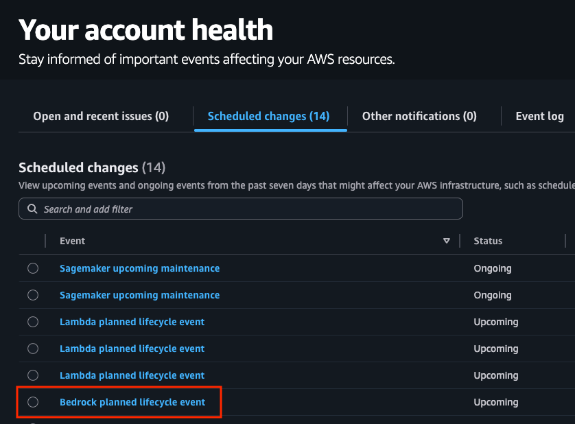
 Saurabh Trikande is a Senior Product Supervisor for Amazon Bedrock and Amazon SageMaker Inference. He’s keen about working with clients and companions, motivated by the objective of democratizing AI. He focuses on core challenges associated to deploying complicated AI purposes, inference with multi-tenant fashions, price optimizations, and making the deployment of generative AI fashions extra accessible. In his spare time, Saurabh enjoys mountaineering, studying about progressive applied sciences, following TechCrunch, and spending time along with his household.
 Melanie Li, PhD, is a Senior Generative AI Specialist Options Architect at AWS based mostly in Sydney, Australia, the place her focus is on working with clients to construct options utilizing state-of-the-art AI/ML instruments. She has been actively concerned in a number of generative AI initiatives throughout APJ, harnessing the facility of LLMs. Previous to becoming a member of AWS, Dr. Li held knowledge science roles within the monetary and retail industries.
 Derrick Choo is a Senior Options Architect at AWS who accelerates enterprise digital transformation by means of cloud adoption, AI/ML, and generative AI options. He focuses on full-stack growth and ML, designing end-to-end options spanning frontend interfaces, IoT purposes, knowledge integrations, and ML fashions, with a selected concentrate on laptop imaginative and prescient and multi-modal programs.
 Jared Dean is a Principal AI/ML Options Architect at AWS. Jared works with clients throughout industries to develop machine studying purposes that enhance effectivity. He’s inquisitive about all issues AI, know-how, and BBQ.
 Julia Bodia is Principal Product Supervisor for Amazon Bedrock.
 Pooja Rao is a Senior Program Supervisor at AWS, main quota and capability administration and supporting enterprise growth for the Bedrock Go-To-Market crew. Outdoors of labor, she enjoys studying, touring, and spending time together with her household.