Home Blog Page 642

A Good Instrument is a Dangerous Management

0

[ad_1]

Right here’s a puzzle for you.
What’s going to occur if we regress some consequence of curiosity on each an endogenous regressor and a sound instrument for that regressor?
I hadn’t thought of this query till 2018, when one in all my undergraduate college students requested it throughout class.
If reminiscence serves, my off-the-cuff reply left a lot to be desired.
5 years later I’m lastly prepared to offer a completely passable reply; higher late than by no means I suppose!

We’ll begin by being a bit extra exact in regards to the setup.
Suppose that (Y) is expounded to (X) based on the next linear causal mannequin [
Y leftarrow alpha + beta X + U
]

the place (beta) is the causal impact of curiosity and (U) represents unobserved causes of (Y) that could be associated to (X).
Now, for any noticed random variable (Z), we will outline
[
V equiv X – (pi_0 + pi_1 Z), quad pi_0 equiv mathbb{E}[X] – pi_1 mathbb{E}[Z], quad pi_1 equiv frac{textual content{Cov}(X,Z)}{textual content{Var}(Z)}.
]

That is the inhabitants linear regression of (X) on (Z).
By building it satisfies (mathbb{E}[V] = textual content{Cov}(Z,V) = 0).
Thus we will write,
[
X = pi_0 + pi_1 Z + V, quad mathbb{E}[V] = textual content{Cov}(Z,V) = 0
]

for any random variables (X) and (Z), just by setting up (V) as described above.
If (pi_1 neq 0), we are saying that (Z) is related.
If (textual content{Cov}(Z,U) = 0), we are saying that (Z) is exogenous.
If (Z) is each related and exogenous, we are saying that it’s a legitimate instrument for (X).

As we’ve outlined it above, (V) is solely a regression residual.
But when (Z) is a sound instrument, it seems that we will consider (V) because the “endogenous half” of (X).
To see why, increase (textual content{Cov}(X,U)) as follows:
[
text{Cov}(X,U) = text{Cov}(pi_0 + pi_1 Z + V, ,U) = pi_1 text{Cov}(Z,U) + text{Cov}(U,V) = text{Cov}(U,V)
]

since we’ve got assumed that (textual content{Cov}(Z,U) = 0).
In phrases, the endogeneity of (X) is exactly the identical factor because the covariance between (U) and (V).

Right here’s a useful mind-set about this.
If (Z) is exogenous then our regression of (X) on (Z) partitions the general variation in (X) into two elements: the “good” (exogenous) variation (pi_1 Z) is uncorrelated with (U), whereas the “dangerous” (endogenous) variation (V) is correlated with (U).
The logic of two-stage least squares is that regressing (Y) on the “good” variation, (pi_1 Z) permits us to get better (beta), the causal impact of curiosity.

Utilizing the mannequin and derivations from above, let’s run a little bit simulation.
To simulate a sound instrument (Z) and an endogenous regressor (X) we will proceed as follows.
First generate unbiased commonplace regular attracts ({Z_i}_{i=1}^n).
Subsequent independently generate pairs of correlated commonplace regular attracts ({(U_i, V_i)}_{i=1}^n) with (textual content{Corr}(U_i, V_i) = rho).
Lastly, set
[
X_i = pi_0 + pi_1 Z_i + V_i quad text{and} quad
Y_i = alpha + beta X_i + U_i
]

for every worth of (i) between (1) and (n).
The next chunk of R code runs this simulation with (n = 5000), (rho = 0.5), (pi_0 = 0.5), (pi_1 = 0.8), (alpha = -0.3) and (beta = 1):

set.seed(1234)
n <- 5000
z <- rnorm(n)

library(mvtnorm)
Rho <- matrix(c(1, 0.5, 
                0.5, 1), 2, 2, byrow = TRUE)
errors <- rmvnorm(n, sigma = Rho)

u <- errors[, 1]
v <- errors[, 2]
x <- 0.5 + 0.8 * z + v
y <- -0.3 + x + u

Within the simulation (Z) is a sound instrument, (X) is an endogenous regressor, and the true causal impact of curiosity equals one.
Utilizing our simulation knowledge, let’s take a look at out three potential estimators:

  • (widehat{beta}_text{OLS}equiv) the slope coefficient from an OLS regression of (Y) on (X).
  • (widehat{beta}_text{IV}equiv) slope coefficient from an IV regression of (Y) on (X) with (Z) as an instrument.
  • (widehat{beta}_{X.Z}equiv) the coefficient on (X) in an OLS regression of (Y) on (X) and (Z).
c(fact = 1,
  b_OLS = cov(x, y) / var(x), 
  b_IV = cov(z, y) / cov(z, x), 
  b_x.z = unname(coef(lm(y ~ x + z))[2])) |> # unname() makes the names prettier!
  spherical(2)
## fact b_OLS  b_IV b_x.z 
##  1.00  1.31  1.01  1.49

As anticipated, OLS is much from the reality whereas IV just about nails it.
Curiously, the regression of y on x and z provides the worst efficiency of all! Is that this only a fluke?
Maybe it’s an artifact of the simulation parameters I selected, or simply dangerous luck arising from some uncommon simulation attracts.
To search out out, we’ll want a bit extra algebra.
However stick with me: the payoff is price it, and there’s not an excessive amount of additional math required!

Regression of (Y) on (X) and (Z)

The coefficient on (X) in a inhabitants linear regression of (Y) on (X) and (Z) is given by
[
beta_{X.Z} = frac{text{Cov}(tilde{X}, Y)}{text{Var}(tilde{X})}
]

the place (tilde{X}) is outlined because the residual in one other inhabitants linear regresasion: the regression of (X) on (Z).
However wait a minute: we’ve already seen this residual!
Above we known as it (V) and used it to put in writing (X = pi_0 + pi_1 Z + V).
Utilizing this equation, together with the linear causal mannequin relating (Y) to (X) and (U), we will re-express (beta_{X.Z}) as
[
begin{align*}
beta_{X.Z} &= frac{text{Cov}(V, Y)}{text{Var}(V)} = frac{text{Cov}(V, alpha + beta X + U)}{text{Var}(V)}
&= frac{text{Cov}(U,V) + betatext{Cov}(V, pi_0 + pi_1 Z + V)}{text{Var}(V)}
&= beta + frac{text{Cov}(U,V)}{text{Var}(V)}
end{align*}
]

since (textual content{Cov}(Z, V) = 0) by building.
We’ve some simulation knowledge at our disposal, so let’s examine this calculation.
Within the simulation (beta = 1) and
[
frac{text{Cov}(U, V)}{text{Var}(V)} = 0.5
]

since (textual content{Var}(U) = textual content{Var}(V) = 1) and (textual content{Cov}(U, V) = 0.5).
Subsequently (beta_{X.Z} = 1.5).
And, certainly, that is nearly precisely the worth of our estimate from our simulation above.

Regression of (Y) on (X) Solely

Thus far so good.
Now what in regards to the “regular” OLS estimator?
A fast calculation provides
[
beta_{text{OLS}} = beta + frac{text{Cov}(X,U)}{text{Var}(X)} = beta + frac{text{Cov}(V,U)}{text{Var}(X)}
]

utilizing the truth that (textual content{Cov}(X,U) = textual content{Cov}(U,V)), as defined above.
Once more, we will examine this in opposition to our simulation outcomes.
We all know that (textual content{Cov}(V,U) = 0.5) and
[
text{Var}(X) = text{Var}(pi_0 + pi_1 Z + V) = pi_1^2 text{Var}(Z) + text{Var}(V) = (0.8)^2 + 1 = 41/25
]

since (Z) and (V) are uncorrelated by building, (textual content{Var}(Z) = textual content{Var}(V) = 1) and (pi_1 = 0.8) within the simulation design.
Therefore, (beta_{textual content{OLS}} = 1 + 25/82 approx 1.305).
Once more, this agrees nearly completely with our simulation.

Evaluating the Outcomes

To summarize, we’ve got proven that
[
beta_{X.Z} = beta + frac{text{Cov}(U,V)}{text{Var}(V)}, quad text{while} quad
beta_{text{OLS}} = beta + frac{text{Cov}(U,V)}{text{Var}(X)}.
]

There is just one distinction between these two expressions: (beta_{X.Z}) has (textual content{Var}(V)) the place (beta_{textual content{OLS}}) has (textual content{Var}(X)).
Returning to our expression for (textual content{Var}(X)) from above,
[
text{Var}(X) = pi_1^2 text{Var}(Z) + text{Var}(V) > text{Var}(V)
]

so long as (pi_1 neq 0) and (textual content{Var}(Z) neq 0).
In different phrases, there may be all the time extra variation in (X) than there may be in (V), since (V) is the “leftover” a part of (X) after regressing on (Z).
As a result of the variances of (X) and (V) seem within the denominators of our expressions from above, it follows that
[
left| text{Cov}(U,V)/text{Var}(V)right| > left| text{Cov}(U,V)/text{Var}(X)right|.
]

In different phrases, (beta_{X.Z}) is all the time farther from the reality than (beta_{OLS}), precisely as we present in our simulation.

In our simulation, (widehat{beta}_{X.Z}) gave a worse estimate of (beta) than (widehat{beta}_{X.Z}).
The derivations from above present that this wasn’t a fluke: including a sound instrument (Z) as an extra management regressor solely makes the bias in our estimated causal impact worse than it was to start with.
This holds for any legitimate instrument and any endogenous regressor in a linear causal mannequin.
I hope you discovered the derivations from above convincing.
Besides, chances are you’ll be questioning if there’s an intuitive rationalization for this phenomenon.
I’m please to tell you that the reply is sure!

In an earlier put up I described the management operate strategy to instrumental variables regression.
That put up confirmed that the coefficient on (X) in a regression of (Y) on (X) and (V) provides the right causal impact.
We don’t know (V), however we will estimate it by regressing (X) on (Z) and saving the residuals.
The logic of a number of regression exhibits that together with (V) as a management regressor “soaks up” the portion of (X) that’s defined by (V).
As a result of (V) represents the “dangerous” (endogenous) variation in (X), this solves our endogeneity drawback.
In impact, (V) captures the unobserved “omitted variables” that play havoc with a naive regression of (Y) on (X).

Now, distinction this with a regression of (Y) on (X) and (Z).
On this case, we absorb the variation in (X) that’s defined by (Z).
However (Z) represents the good (exogenous) variation in (X)!
Absorbing this variation leaves solely the dangerous variation behind, making our endogeneity drawback worse than it was to start with.
On this instance, (Z) is what is called a dangerous management, a management regressor that makes issues worse quite than higher.
A standard piece of recommendation for avoiding dangerous controls is to solely embrace management regressors which can be correlated with (X) and (Y) however are not themselves attributable to (Z).
The instance on this put up exhibits that this recommendation unsuitable.
Right here (Z) isn’t attributable to (X), and is correlated with each (X) and (Y).
Nonetheless, it’s a dangerous management
In brief, a sound instrument offers a strong technique to perform causal inference from observational knowledge, however provided that you utilize it in the precise method.
An excellent instrument is a foul management!

[ad_2]

Serving to scientists run complicated knowledge analyses with out writing code | MIT Information

0

[ad_1]

As prices for diagnostic and sequencing applied sciences have plummeted in recent times, researchers have collected an unprecedented quantity of information round illness and biology. Sadly, scientists hoping to go from knowledge to new cures usually require assist from somebody with expertise in software program engineering.

Now, Watershed Bio helps scientists and bioinformaticians run experiments and get insights with a platform that lets customers analyze complicated datasets no matter their computational abilities. The cloud-based platform gives workflow templates and a customizable interface to assist customers discover and share knowledge of every kind, together with whole-genome sequencing, transcriptomics, proteomics, metabolomics, high-content imaging, protein folding, and extra.

“Scientists wish to be taught in regards to the software program and knowledge science elements of the sphere, however they don’t wish to grow to be software program engineers writing code simply to grasp their knowledge,” co-founder and CEO Jonathan Wang ’13, SM ’15 says. “With Watershed, they don’t should.”

Watershed is being utilized by giant and small analysis groups throughout business and academia to drive discovery and decision-making. When new superior analytic strategies are described in scientific journals, they are often added to Watershed’s platform instantly as templates, making cutting-edge instruments extra accessible and collaborative for researchers of all backgrounds.

“The information in biology is rising exponentially, and the sequencing applied sciences producing this knowledge are solely getting higher and cheaper,” Wang says. “Coming from MIT, this subject was proper in my wheelhouse: It’s a troublesome technical downside. It’s additionally a significant downside as a result of these persons are working to deal with ailments. They know all this knowledge has worth, however they wrestle to make use of it. We wish to assist them unlock extra insights quicker.”

No code discovery

Wang anticipated to main in biology at MIT, however he rapidly obtained excited by the probabilities of constructing options that scaled to hundreds of thousands of individuals with laptop science. He ended up incomes each his bachelor’s and grasp’s levels from the Division of Electrical Engineering and Pc Science (EECS). Wang additionally interned at a biology lab at MIT, the place he was stunned how gradual and labor-intensive experiments had been.

“I noticed the distinction between biology and laptop science, the place you had these dynamic environments [in computer science] that allow you to get suggestions instantly,” Wang says. “At the same time as a single individual writing code, you may have a lot at your fingertips to play with.”

Whereas engaged on machine studying and high-performance computing at MIT, Wang additionally co-founded a excessive frequency buying and selling agency with some classmates. His group employed researchers with PhD backgrounds in areas like math and physics to develop new buying and selling methods, however they rapidly noticed a bottleneck of their course of.

“Issues had been transferring slowly as a result of the researchers had been used to constructing prototypes,” Wang says. “These had been small approximations of fashions they might run regionally on their machines. To place these approaches into manufacturing, they wanted engineers to make them work in a high-throughput approach on a computing cluster. However the engineers didn’t perceive the character of the analysis, so there was a variety of forwards and backwards. It meant concepts you thought might have been carried out in a day took weeks.”

To unravel the issue, Wang’s group developed a software program layer that made constructing production-ready fashions as simple as constructing prototypes on a laptop computer. Then, a couple of years after graduating MIT, Wang observed applied sciences like DNA sequencing had grow to be low cost and ubiquitous.

“The bottleneck wasn’t sequencing anymore, so individuals stated, ‘Let’s sequence all the things,’” Wang remembers. “The limiting issue turned computation. Folks didn’t know what to do with all the information being generated. Biologists had been ready for knowledge scientists and bioinformaticians to assist them, however these individuals didn’t all the time perceive the biology at a deep sufficient degree.”

The state of affairs appeared acquainted to Wang.

“It was precisely like what we noticed in finance, the place researchers had been making an attempt to work with engineers, however the engineers by no means totally understood, and also you had all this inefficiency with individuals ready on the engineers,” Wang says. “In the meantime, I discovered the biologists are hungry to run these experiments, however there may be such an enormous hole they felt they needed to grow to be a software program engineer or simply concentrate on the science.”

Wang formally based Watershed in 2019 with doctor Mark Kalinich ’13, a former classmate at MIT who’s now not concerned in day-to-day operations of the corporate.

Wang has since heard from biotech and pharmaceutical executives in regards to the rising complexity of biology analysis. Unlocking new insights more and more includes analyzing knowledge from whole genomes, inhabitants research, RNA sequencing, mass spectrometry, and extra. Growing personalised therapies or choosing affected person populations for a scientific examine may also require large datasets, and there are new methods to investigate knowledge being printed in scientific journals on a regular basis.

In the present day, corporations can run large-scale analyses on Watershed with out having to arrange their very own servers or cloud computing accounts. Researchers can use ready-made templates that work with all the most typical knowledge sorts to speed up their work. Widespread AI-based instruments like AlphaFold and Geneformer are additionally obtainable, and Watershed’s platform makes sharing workflows and digging deeper into outcomes simple.

“The platform hits a candy spot of usability and customizability for individuals of all backgrounds,” Wang says. “No science is ever really the identical. I keep away from the phrase product as a result of that suggests you deploy one thing and you then simply run it at scale ceaselessly. Analysis isn’t like that. Analysis is about developing with an concept, testing it, and utilizing the end result to provide you with one other concept. The quicker you’ll be able to design, implement, and execute experiments, the quicker you’ll be able to transfer on to the following one.”

Accelerating biology

Wang believes Watershed helps biologists sustain with the newest advances in biology and accelerating scientific discovery within the course of.

“In case you will help scientists unlock insights not a little bit bit quicker, however 10 or 20 occasions quicker, it may actually make a distinction,” Wang says.

Watershed is being utilized by researchers in academia and in corporations of all sizes. Executives at biotech and pharmaceutical corporations additionally use Watershed to make choices about new experiments and drug candidates.

“We’ve seen success in all these areas, and the frequent thread is individuals understanding analysis however not being an knowledgeable in laptop science or software program engineering,” Wang says. “It’s thrilling to see this business develop. For me, it’s nice being from MIT and now to be again in Kendall Sq. the place Watershed is predicated. That is the place a lot of the cutting-edge progress is going on. We’re making an attempt to do our half to allow the way forward for biology.”

[ad_2]

A practitioner’s primer on deterministic software modernization

0

[ad_1]

// Supply code snippet
// The consumer's identify
personal String identify = "Java";

// LST illustration
J.VariableDeclarations | "// The consumer's namenprivate String identify = "Java""
|---J.Modifier | "personal"
|---J.Identifier | "String"
---J.VariableDeclarations.NamedVariable | "identify = "Java""
    |---J.Identifier | "identify"
    ---J.Literal | ""Java""

Recipes work with many various file varieties together with XML or YAML to switch issues like Maven POMs or different configuration information. In addition they can create new information when wanted as a part of migrations. However recipes don’t even have to switch code in any respect. A strong characteristic and good thing about the wealthy knowledge from the LST is that they could simply collect knowledge and insights, analyzing code bases to generate knowledge tables for use for studies, metrics, or visualizations that assist groups perceive their code earlier than making adjustments.

Testing recipes: Deterministic and dependable

OpenRewrite’s deterministic nature makes recipes simple to check. Right here’s how easy it’s to visualise the adjustments a recipe ought to make, and to confirm it really works appropriately:

@Check
void migrateJUnitTest() {
    rewriteRun(
        // The recipe to check
        new MigrateToJUnit5(),
        
        // Earlier than: JUnit 4 code
        java("""
            import org.junit.Check;
            
            public class MyTest {
                @Check
                public void testSomething() {}
            }
            """),
            
        // After: Anticipated JUnit 5 outcome
        java("""
            import org.junit.jupiter.api.Check;
            
            public class MyTest {
                @Check
                public void testSomething() {}
            }
            """)
    );
}

This check framework validates that the recipe produces precisely the anticipated output—no extra, no much less. As a result of recipes are deterministic, the identical enter all the time produces the identical outcome, making them dependable and testable at scale.

[ad_2]

Run LM Studio Fashions Domestically in your Machine

[ad_1]

Introduction

LM Studio makes it extremely straightforward to run and experiment with open-source giant language fashions (LLMs) completely in your native machine, with no web connection or cloud dependency required. You’ll be able to obtain a mannequin, begin chatting, and discover responses whereas sustaining full management over your knowledge.

However what if you wish to transcend the native interface?

Let’s say your LM Studio mannequin is up and working domestically, and now you wish to name it from one other app, combine it into manufacturing, share it securely along with your crew, or join it to instruments constructed across the OpenAI API.

That’s the place issues get difficult. LM Studio runs fashions domestically, nevertheless it doesn’t natively expose them by means of a safe, authenticated API. Setting that up manually would imply dealing with tunneling, routing, and API administration by yourself.

That’s the place Clarifai Native Runners are available. Native Runners allow you to serve AI fashions, MCP servers, or brokers immediately out of your laptop computer, workstation, or inside server, securely and seamlessly by way of a public API. You don’t want to add your mannequin or handle any infrastructure. Run it domestically, and Clarifai handles the API, routing, and integration.

As soon as working, the Native Runner establishes a safe connection to Clarifai’s management airplane. Any API request despatched to your mannequin is routed to your machine, processed domestically, and returned to the consumer. From the skin, it behaves like a Clarifai-hosted mannequin, whereas all computation occurs in your native {hardware}.

With Native Runners, you may:

  • Run fashions by yourself {hardware}
    Use laptops, workstations, or on-prem servers with full entry to native GPUs and system instruments.

  • Preserve knowledge and compute personal
    Keep away from importing something. That is helpful for regulated environments and delicate tasks.

  • Skip infrastructure setup
    No have to construct and host your individual API. Clarifai gives the endpoint, routing, and authentication.

  • Prototype and iterate shortly
    Take a look at fashions in actual pipelines with out deployment delays. Examine requests and outputs stay.

  • Hook up with native recordsdata and personal APIs
    Let fashions entry your file system, inside databases, or OS assets with out exposing your surroundings.

Now that the advantages are clear, let’s see tips on how to run LM Studio fashions domestically and expose them securely by way of an API.

Operating LM Studio Fashions Domestically

The LM Studio Toolkit within the Clarifai CLI lets you initialize, configure, and run LM Studio fashions domestically whereas exposing them by means of a safe public API. You’ll be able to take a look at, combine, and iterate immediately out of your machine with out standing up infrastructure.

Notice: Obtain and hold LM Studio open when working the Native Runner. The runner launches and communicates with LM Studio by means of its native port to load, serve, and run mannequin inferences.

Step 1: Stipulations

  1. Set up the Clarifai bundle and CLI

  1. Log in to Clarifai

Observe the prompts to enter your Person ID and Private Entry Token (PAT). If you happen to need assistance acquiring these, seek advice from the documentation.

Step 2: Initialize a Mannequin

Use the Clarifai CLI to initialize and configure an LM Studio mannequin domestically. Solely fashions obtainable within the LM Studio Mannequin Catalog and in GGUF format are supported.

Initialize the default instance mannequin

By default, this creates a mission for the LiquidAI/LFM2-1.2B LM Studio mannequin in your present listing.

If you wish to work with a selected mannequin reasonably than the default LiquidAI/LFM2-1.2B, you should utilize the --model-name flag to specify the total mannequin title. See the total record of all fashions right here.

Notice: Some fashions are giant and require important reminiscence. Guarantee your machine meets the mannequin’s necessities earlier than initializing.

Now, when you run the above command, the CLI will scaffold the mission for you. The generated listing construction will appear to be this:

  • mannequin.py comprises the logic that calls LM Studio’s native runtime for predictions.
  • config.yaml defines metadata, compute traits, and toolkit settings.
  • necessities.txt lists Python dependencies.

Step 3: Customise mannequin.py

The scaffold consists of an LMstudioModelClass that extends OpenAIModelClass. It defines how your Native Runner interacts with LM Studio’s native runtime.

Key strategies:

  • load_model() – Launches LM Studio’s native runtime, hundreds the chosen mannequin, and connects to the server port utilizing the OpenAI-compatible API interface.

  • predict() – Handles single-prompt inference with non-obligatory parameters resembling max_tokens, temperature, and top_p. Returns the whole mannequin response.

  • generate() – Streams generated tokens in actual time for interactive or incremental outputs.

You need to use these implementations as-is or modify them to align along with your most popular request and response buildings.

Step 4: Configure config.yaml

The config.yaml file defines mannequin identification, runtime, and compute metadata to your LM Studio Native Runner:

  • mannequin – Contains id, user_id, app_id, and model_type_id (for instance, text-to-text).

  • toolkit – Specifies lmstudio because the supplier. Key fields embody:

    • mannequin – The LM Studio mannequin to make use of (e.g., LiquidAI/LFM2-1.2B).

    • port – The native port the LM Studio server listens on.

    • context_length – Most context size for the mannequin.

  • inference_compute_info – For Native Runners, that is principally non-obligatory, as a result of the mannequin runs completely in your native machine and makes use of your native CPU/GPU assets. You’ll be able to go away defaults as-is. If you happen to plan to deploy the mannequin on Clarifai’s devoted compute, you may specify CPU/reminiscence limits, variety of accelerators, and GPU sort to match your mannequin necessities.

  • build_info – Specifies the Python model used for the runtime (e.g., 3.12).

Lastly, the necessities.txt file lists Python dependencies your mannequin wants. Add any additional packages required by your logic.

Step 5: Begin the Native Runner

Begin a Native Runner that connects to LM Studio’s runtime:

If contexts or defaults are lacking, the CLI will immediate you to create them. This ensures compute contexts, nodepools, and deployments are set in your configuration.

After startup, you’ll obtain a public Clarifai URL to your native mannequin. Requests despatched to this endpoint route securely to your machine, run by means of LM Studio, then return to the consumer.

Run Inference with Native Runner

As soon as your LM Studio mannequin is working domestically and uncovered by way of the Clarifai Native Runner, you may ship inference requests from anyplace utilizing the OpenAI-compatible API or the Clarifai SDK.

OpenAI-Appropriate API

Clarifai Python SDK

You too can experiment with generate() technique for real-time streaming.

Conclusion

Native Runners offer you full management over the place your fashions execute with out sacrificing integration, safety, or flexibility. You’ll be able to prototype, take a look at, and serve actual workloads by yourself {hardware}, whereas Clarifai handles routing, authentication, and the general public endpoint.

You’ll be able to strive Native Runners at no cost with the Free Tier, or improve to the Developer Plan at $1 per 30 days for the primary 12 months to attach as much as 5 Native Runners with limitless hours.


[ad_2]

Ray-Ban Meta Gen 2 overview: You do not want a show

0

[ad_1]

Why you may belief Android Central


Our knowledgeable reviewers spend hours testing and evaluating services so you may select the perfect for you. Discover out extra about how we take a look at.

After I reviewed the unique Ray-Ban Meta glasses, I defined how a lot I preferred them, however that others may skip them due to the Meta connection and privateness issues. As a substitute, they grew to become the world’s best-selling good glasses. Ray-Ban/Oakley maker EssilorLuxottica is thriving because of AI glasses gross sales, heading in the right direction to make 10 million models subsequent yr to satisfy demand.

My Gen 2 overview will deal with two sorts of folks: the thousands and thousands of Gen 1 patrons questioning whether or not these new glasses are sufficient to justify an improve, and good glasses skeptics questioning whether or not to hop on the Ray-Ban practice.

How AI can enhance storm surge forecasts to assist save lives

0

[ad_1]

This text was initially printed at The Dialog. The publication contributed the article to House.com’s Knowledgeable Voices: Op-Ed & Insights.

Hurricanes are America’s most damaging pure hazards, inflicting extra deaths and property harm than every other sort of catastrophe. Since 1980, these highly effective tropical storms have executed greater than US$1.5 trillion in harm and killed greater than 7,000 folks.

Dempster’s evaluation and donkeys – Statisfaction

0

[ad_1]

This put up is about estimating the parameter of a Bernoulli distribution from observations, within the “Dempster” or “Dempster–Shafer” method, which is a generalization of Bayesian inference. I’ll recall what this strategy is about, and describe a Gibbs sampler to carry out the computation. Intriguingly the related Markov chain occurs to be equal to the so-called “donkey stroll” (not this one), as identified by Guanyang Wang and Persi Diaconis.

Denote the observations, or “coin flips”, by (x_1,ldots,x_N)in{0,1}^N. The mannequin stipulates that x_n = 1(u_n < theta), the place u_n are unbiased Uniform(0,1) variables, and theta in (0,1) is the parameter to be estimated. That’s, x_n = 1 if some uniform lands beneath theta, which certainly happens with likelihood theta, in any other case x_n = 0. We’ll name the uniform variables “auxiliary”, and denote by N_0,N_1 the counts of “0” and “1”, with N_0 + N_1 = N.

In a Bayesian strategy, we’d specify a previous distribution on the parameter; for instance a Beta prior would result in a Beta posterior on theta. The auxiliary variables would play no position; aside maybe in Approximate Bayesian Computation. In Dempster’s strategy, we are able to keep away from the specification of a previous, and as an alternative, and “switch” the randomness from the auxiliary variables to a distribution of subsets of parameters; see ref [1] beneath. Let’s see how this works.

Given observations (x_1,ldots,x_N)in{0,1}^N, there are auxiliary variables (u_1,ldots,u_N) which are suitable with the observations, within the sense that there exists some theta such that forall nin{1,ldots,n} ; x_n = 1(u_n < theta). And there are different configurations of (u_1,ldots,u_N) that aren’t suitable. If we denote by mathcal{I}_0 the indices nin {1,ldots,N} akin to an noticed x_n = 0, and likewise for mathcal{I}_1, we are able to see that there exists some “possible” theta solely when max_{ninmathcal{I}_1} u_n < min_{ninmathcal{I}_0} u_n. In that case the possible theta are within the interval (max_{ninmathcal{I}_1} u_n, min_{ninmathcal{I}_0} u_n). The next diagram illustrates this with N_0  = 2, N_1 = 3.

How will we acquire the distribution of those units mathcal{F}(u), beneath the Uniform distribution of uin [0,1]^N and conditioning on mathcal{F}(u)neq emptyset? We may draw N uniforms, sorted in growing order, and report the interval between the N_1-th and the (N_1+1)-th values (Part 4 in [1]). However that might be no enjoyable, so allow us to think about a Gibbs sampler as an alternative (taken from [4]). We’ll pattern the auxiliary variables uniformly, conditional upon mathcal{F}(u)neq emptyset, and we’ll proceed by sampling the variables u_n listed by mathcal{I}_0 given the variables listed by mathcal{I}_1, and vice versa. The joint distribution of all of the variables has density proportional to

1(forall n ; u_n in (0,1) quad text{and} quad max_{ninmathcal{I}_1} u_n < min_{ninmathcal{I}_0} u_n).

From this joint density we are able to work out the conditionals. We are able to then categorical the Gibbs updates by way of the endpoints of the interval mathcal{F}(u). Particularly, writing the endpoints at iteration t as (Y^{(t)},Z^{(t)}), the Gibbs sampler is equal to:

  • Sampling Y^{(t)} = Z^{(t-1)} times text{Beta}(N_1,1).
  • Sampling Z^{(t)} = Y^{(t)} + (1-Y^{(t)}) times text{Beta}(1,N_2).

That is precisely the mannequin of Buridan’s donkey in refs [2,3] beneath. The concept is that the donkey, being each hungry and thirsty however not having the ability to select between the water and the hay, takes a step in both course alternatively.

The donkey stroll has been generalized to greater dimensions in [3], and in a way our Gibbs sampler in [4] can be a generalization to greater dimensions… it’s not clear whether or not these two generalizations are the identical or not. So I’ll depart that dialogue for one more day.

A couple of remarks to wrap up.

  • It’s a function of Dempster’s strategy that it yields random subsets of parameters relatively than singletons as customary Bayesian evaluation. Dempster’s strategy is a generalization of Bayes: if we specify a regular prior and apply “Dempster’s rule of mixture” we retrieve customary Bayes.
  • What will we do with these random intervals mathcal{F}(u), as soon as we acquire them? We are able to compute the proportion of them that intersects/is contained in a set of curiosity, for instance the set {theta > 1/2}, and these proportions are reworked into measures of settlement, disagreement or indeterminacy relating to the set of curiosity, versus posterior chances in customary Bayes.
  • Dempster’s estimates rely upon the selection of sampling mechanism and related auxiliary variables, which is matter of many discussions in that literature.
  • In a earlier put up I described an equivalence between the sampling mechanism thought of in [1] when there are greater than two classes, and the Gumbel-max trick… plainly the Dempster’s strategy has numerous intriguing connections.

References:

  • [1] Arthur P. Dempster, New Strategies for Reasoning In direction of Posterior Distributions Primarily based on Smple Knowledge, 1966. [link]
  • [2] Jordan Stoyanov & Christo Pirinsky, Random motions, lessons of ergodic Markov chains and beta distributions, 2000. [link]
  • [3] Gérard Letac, Donkey stroll and Dirichlet distributions, 2002. [link]
  • [4] Pierre E Jacob, Ruobin Gong, Paul T. Edlefsen & Arthur P. Dempster, A Gibbs sampler for a category of random convex polytopes, 2021. [link]

[ad_2]

Massive Animal Illness Outbreaks Across the World

0

[ad_1]

Bovine Spongiform Encephalopathy (BSE), extra generally referred to as mad cow illness, has left a long-lasting mark on the agricultural world.

This insidious disease-causing agent, which ends up in the gradual breakdown of the central nervous system (CNS) in cattle, is called for the sponge-like look of BSE-infected mind tissue beneath a microscope [1,2].

Illness overview

BSE is a progressive neurodegenerative illness attributable to a prion [2].

A prion is a kind of irregular, misfolded protein that may trigger illness by inducing different regular proteins to misfold in an identical manner. This results in mind injury and neurodegenerative issues. The BSE prion wreaks havoc on the CNS of affected cattle [1, 3].

Main outbreaks

The late Nineteen Eighties within the UK marked the start of a devastating illness outbreak of BSE. Contaminated cows displayed alarming signs reminiscent of nervousness, hypersensitivity, and unsteadiness.

By the early Nineteen Nineties, the illness had unfold considerably, peaking in 1992 with 37,280 confirmed circumstances.

Contaminated feed, notably meat and bone meal (MBM), was recognized as the first supply for the unfold of the illness [2].

Affect

Between 1986 and 2001, over 4.5 million cattle had been culled within the UK alone, leading to monumental financial losses. The human toll included over 178 deaths from variant Creutzfeldt-Jakob Illness (vCJD) between 1995 and 2016 [2,3].

The disaster additionally led to a major lack of shopper confidence in British beef, prompting worldwide bans on imports [2].

Challenges and future methods for prevention

The absence of a vaccine for BSE underscores the necessity for preventive measures, reminiscent of destroying contaminated animals and rigorous feed controls. The distinctive nature of prions continues to problem illness management efforts [4].


[ad_2]

GARCH vs. GJR-GARCH Fashions in Python for Volatility Forecasting

0

[ad_1]

By Manusha Rao

You might have seen that markets typically stay calm for weeks after which swing wildly for a couple of days. That’s volatility in motion. It measures how a lot costs transfer—and it’s a giant deal in buying and selling and investing as a result of it displays danger. However right here’s the catch: estimating volatility is not simple.

A 2% drop typically sparks extra headlines than a 2% achieve. That’s uneven volatility—and it is what conventional fashions miss.

Enter the GJR-GARCH mannequin!


Conditions

This weblog focuses on volatility forecasting utilizing the GJR-GARCH mannequin, with a sensible Python implementation based mostly on the NIFTY 50 index. It explains the idea of uneven volatility, the way it differs from the standard GARCH mannequin, and supplies instruments for evaluating forecast high quality by visualizations and diagnostics.

To know and apply the GJR-GARCH mannequin successfully, it is necessary to start out with the fundamentals of time sequence evaluation. Start with Introduction to Time Collection to get accustomed to development, seasonality, and autocorrelation. For those who’re exploring how deep studying compares to conventional fashions, learn Time Collection vs LSTM Fashions for a conceptual comparability.

Since GARCH and GJR-GARCH fashions depend on stationary time sequence, examine Stationarity to discover ways to put together your knowledge. Improve this data by studying The Hurst Exponent for insights into long-term reminiscence in time sequence and Imply Reversion in Time Collection for understanding mean-reverting conduct—typically linked with volatility clusters.

You must also be accustomed to the ARMA household of fashions, that are foundational to ARIMA and GARCH. For this, seek advice from the ARMA Mannequin Information and its companion weblog ARMA Implementation in Python. Lastly, to understand the terminology and idea behind GARCH, the Quantra glossary entries on GARCH and Volatility Forecasting utilizing GARCH are important assets.

On this weblog, we’ll discover the next:


Distinction between GARCH and GJR-GARCH fashions

The GARCH mannequin captures volatility clustering however assumes that optimistic and damaging shocks have a symmetric impact on future volatility. In distinction, the GJR-GARCH mannequin accounts for asymmetry by giving extra weight to damaging shocks, which displays the leverage impact generally noticed in monetary markets. Why? As a result of worry drives quicker and stronger reactions than optimism in monetary markets.

GJR-GARCH introduces a further parameter that prompts when previous returns are damaging. This makes it extra appropriate for modelling real-world inventory knowledge, the place dangerous information sometimes causes larger volatility.

For instance, in the course of the COVID-19 market crash in March 2020, the NIFTY 50 noticed sharp declines and sudden spikes in volatility pushed by panic promoting proven under.

Supply: TradingView

A GARCH mannequin would understate this asymmetry, whereas GJR-GARCH captures the heightened volatility following damaging shocks extra precisely. Total, GJR-GARCH is a extra versatile and sensible extension of the usual GARCH mannequin.


A short take a look at the GARCH mannequin

The GARCH (Generalized Autoregressive Conditional Heteroskedasticity) mannequin is a well-liked statistical software for forecasting monetary market volatility. Developed by Tim Bollerslev in 1986 as an extension of the ARCH mannequin, GARCH captures the tendency of volatility to cluster over time—which means intervals of excessive volatility are typically adopted by intervals of excessive volatility, and intervals of calm are adopted by extra intervals of calm.

In essence, the GARCH mannequin assumes that at present’s volatility relies upon not solely on previous squared returns (as in ARCH) but additionally on previous volatility estimates. This makes it particularly helpful for modelling time sequence knowledge with altering variance, resembling asset returns.

The overall equation for a GARCH(p, q) mannequin, which fashions conditional variance, is:

ARCH & GARCH

  • σ2t: Represents the conditional variance of the time sequence at time ‘t’.
  • ω: A relentless time period representing the long-run or common variance.
  • Σ(αi * ε2t−i): The ARCH part, capturing the impact of previous squared errors on the present variance.
  • Σ(βj * σ2t−j): The GARCH part, capturing the impact of previous conditional variances on the present variance.

Word: GARCH(1,1) is the only type of the GARCH mannequin:


σ2t = ω + α1 ε2t−1 + β1 σ2t−1

With solely three parameters (fixed, ARCH time period, and GARCH time period), it is simple to estimate and interpret—perfect for monetary knowledge the place too many parameters will be unstable.


Introduction to the GJR-GARCH mannequin

The GJR-GARCH mannequin, proposed by Glosten, Jagannathan, and Runkle (1993), is an extension of the usual GARCH mannequin designed to seize the uneven results of stories on volatility.

The GJR-GARCH(1,1) components is given by:


σ2t = ω + α1 ε2t−1 + γ ε2t−1 It−1 + β1 σ2t−1

The place,

γ : Represents the extra influence of damaging shocks (leverage impact)


ε2t−1 It−1

: Represents the indicator perform that prompts when the earlier return shock is damaging

Interpretation:

  • When the earlier shock
    εt−1
    is optimistic:
    σt2 = ω + α εt−12 + β σt−12
  • When the earlier shock
    εt−1
    is damaging:
    σt2 = ω + (α + γ) εt−12 + β σt−12
  • So, damaging shocks enhance volatility extra by the quantity
    γ

Now that we perceive the GJR-GARCH mannequin components and its instinct, let’s implement it in Python. We’ll use the arch bundle, which presents a easy but highly effective interface to specify and estimate GARCH-family fashions. Utilizing historic NIFTY 50 returns knowledge, we’ll match a GJR-GARCH(1,1) mannequin, generate rolling volatility forecasts, and consider how effectively the mannequin captures market conduct, particularly throughout turbulent intervals.


Volatility Forecasting on NIFTY 50 Utilizing GJR-GARCH in Python

Step 1: Import the mandatory libraries

The tqdm library is used to indicate a progress bar when your code is doing one thing that takes time — like working a loop with loads of steps.

It helps you see how a lot is completed and the way a lot is left, so that you don’t should guess in case your code continues to be working or caught.

Step 2: Obtain NIFTY50 knowledge

Right here we’re utilizing NIFTY 50 knowledge from 2020 to 2025.

Nifty 50 historical data

Subsequent, calculate the every day log returns and specific in share phrases. Fashions like GARCH work higher when the enter numbers aren’t too tiny (like 0.0012), as very small values could make it more durable for the optimizer to converge throughout mannequin becoming.

Step 3: Specify the GJR-GARCH mannequin

To mannequin a GJR-GARCH mannequin in Python,the arch bundle is used. Use Scholar’s t-distribution for residuals, which captures fats tails typically noticed in monetary returns. Be happy to make use of the distribution that most closely fits your buying and selling wants or knowledge distribution.

Right here,

p = 1

Variety of lags of previous squared returns (ARCH time period)

o = 1

Variety of lags for asymmetry time period – this allows the GJR-GARCH (or GARCH with leverage impact)

q = 1

Variety of lags of previous variances (GARCH time period)

Step 4: Match the mannequin

The output is as follows:

Model result
  • The ARCH time period (alpha[1]), which measures the influence of previous shocks, is important on the 5% degree, although comparatively small (0.0123).
  • The GARCH time period (beta[1]) is excessive at 0.9052, implying that volatility is extremely persistent over time.
  • The leverage impact (gamma[1] = 0.1330) is important, confirming the presence of asymmetry—damaging shocks enhance volatility greater than optimistic ones, a standard characteristic in fairness market knowledge.
  • The estimated levels of freedom (nu = 7.6) for the Scholar’s t-distribution recommend the info displays fats tails, justifying the selection of this distribution to seize excessive returns extra precisely.

Step 5: Residual diagnostics

This block of code is for residual diagnostics after becoming your GJR-GARCH mannequin. It helps you visually assess how effectively the mannequin has captured volatility dynamics.

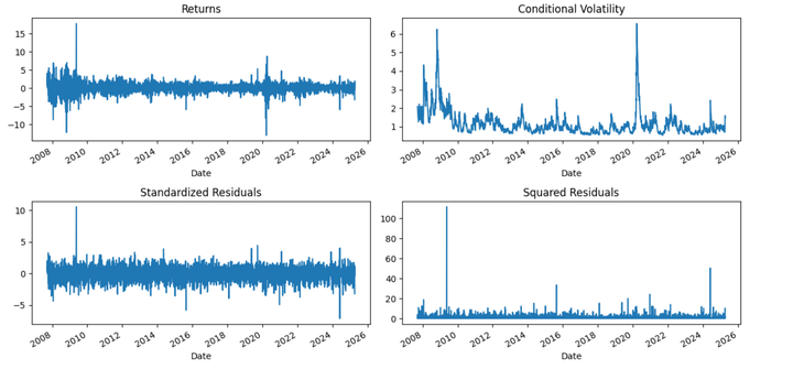
Residual diagnostics

The GJR-GARCH mannequin performs effectively in capturing volatility dynamics throughout main market occasions, particularly intervals of monetary misery. Notable spikes in conditional volatility are noticed in the course of the 2008 world monetary disaster and the 2020 COVID-19 pandemic. The asymmetry part (gamma) performs a key function right here, amplifying volatility predictions in response to damaging returns—mirroring real-world investor conduct the place worry and dangerous information drive sharper market reactions than optimism.

Step 6: Make rolling forecasts of volatility

A extra sensible strategy to forecast volatility is to make one-step-ahead predictions utilizing data accessible as much as time t, after which replace the mannequin in actual time as every new knowledge level turns into accessible (i.e., as t progresses to t+1, t+2, and so on.). In easy phrases, every day we incorporate the most recent noticed return to forecast the subsequent day’s volatility.

Right here we take practice the mannequin on 500 days of previous returns, to forecast 1-day forward volatility, repeated every day.

Now you’d wish to examine GARCH’s 1-day forecast to some observable precise volatility.

The standard methodology is to compute realized every day volatility as a rolling commonplace deviation.

Nevertheless, in case you’re forecasting for 1 day, the realized volatility you must ideally examine it to is:

the precise return (i.e., squared return of the subsequent day), or a smoothed proxy like a 5-day rolling commonplace deviation (if you wish to take away noise).

As illustrated within the plot under, intervals of elevated market uncertainty, resembling mid-2024, exhibit vital spikes within the 1-day forward forecasted volatility, reflecting heightened danger notion. Conversely, calmer intervals like early 2023 present lowered volatility expectations. This strategy permits merchants and danger managers to adaptively regulate publicity and hedging methods in response to anticipated market situations.

The GJR-GARCH mannequin proves particularly precious for its means to react sensitively to draw back shocks. It’s a strong software for short-term volatility forecasting in index-level knowledge just like the NIFTY 50 or inventory knowledge.

Actual vs forecasted

Now allow us to examine the correlation between the realized and forecasted volatility.

Output:

Correlation between Forecasted and Realized Volatility: 0.7443

The noticed correlation of 0.74 between the 5-day rolling realized volatility and the GJR-GARCH forecasted volatility signifies that the mannequin successfully captures the dynamics of market volatility.

Particularly, the GJR-GARCH mannequin, which accounts for uneven responses to optimistic and damaging shocks (i.e., volatility reacts extra to damaging information), aligns effectively with the precise realized volatility. A robust correlation like this means that the mannequin can forecast intervals of excessive or low volatility in a directionally correct method.


Conclusion

Market volatility isn’t simply numbers—it displays human psychology. The GJR-GARCH mannequin goes a step past conventional volatility estimators by recognizing that worry has a stronger market influence than optimism. By modelling this behaviour explicitly, it supplies a extra correct and behaviourally sound option to forecast volatility in varied belongings.


Subsequent Steps

When you’re snug with the GARCH household, you possibly can transfer on to extra complicated volatility modeling strategies. A very good subsequent learn is Time-Various-Parameter VAR (TVP-VAR), which introduces fashions that deal with stochastic volatility and structural modifications over time.

You too can discover ARFIMA fashions for dealing with long-memory processes, that are frequent in monetary market volatility. Understanding these fashions will show you how to create extra strong, adaptable forecasting methods.

To develop efficient buying and selling methods, transcend modeling. Mix your GJR-GARCH insights with sensible strategies from Technical Evaluation to detect developments and momentum, use Buying and selling Threat Administration to guard in opposition to losses, discover Pairs Buying and selling for market-neutral methods, and perceive Market Microstructure to account for execution and liquidity dynamics.

Lastly, for a structured and complete journey into algorithmic buying and selling, think about enrolling within the Govt Programme in Algorithmic Buying and selling (EPAT). EPAT covers superior subjects resembling stationarity, ACF/PACF, ARIMA, ARCH, GARCH, and extra, with sensible coaching in Python technique growth, statistical arbitrage, and alternate knowledge. It’s the right subsequent step for these prepared to use their quantitative expertise in actual markets.


File within the obtain:

GJR GARCH Python Pocket book


Disclaimer: All investments and buying and selling within the inventory market contain danger. Any resolution to position trades within the monetary markets, together with buying and selling in inventory or choices or different monetary devices is a private resolution that ought to solely be made after thorough analysis, together with a private danger and monetary evaluation and the engagement {of professional} help to the extent you consider needed. The buying and selling methods or associated data talked about on this article is for informational functions solely.

[ad_2]

Prime 5 Newbie-Pleasant Programs to Degree Up with Google Abilities

0

[ad_1]

The development for AI upskilling goes on, as the newest gem from the home of Google drops. With the phrases, “Say Hey to Google Abilities,” the corporate has introduced its new initiative that’s meant to upskill folks in AI. It solely is sensible, with AI being the go-to phrase within the job trade. Abilities like these could make or break a deal (hiring). Curiously sufficient, now you’ll be able to be taught straight from Google’s personal ecosystem.

Every of the Google programs provide you with guided labs, sensible duties, and a talent badge you’ll be able to flash wherever, which signifies that you don’t want years of expertise. Simply curiosity and a laptop computer. Consider this platform as a launchpad. You decide a course, you construct a talent, and also you stack real-world credentials.

This text breaks down the highest programs on Google Abilities for absolute newbies. No advanced math. No AI principle. Simply abilities that make you helpful at work from Day One.

Able to degree up? Let’s dive in.

What’s Google Abilities?

Google Abilities is your direct line to sensible studying.

With none form of gatekeeping or infinite principle, Google Abilities permits you to be taught actual abilities by means of guided labs.

The platform bundles newbie paths throughout information, cloud, AI, and office instruments. Each course comes with hands-on workout routines and ends with a Google Ability Badge, principally a proof that you simply truly did the work.

These aren’t generic MOOCs. They’re constructed by Google’s personal product and cloud groups. Which means you be taught the precise instruments used inside international companies.

When you’re new to tech, that is the place you begin. And sure, a lot of the prime programs on Google Abilities are free to start.

Subsequent, let’s have a look at why these newbie abilities truly matter.

Why These Newbie Abilities Matter?

Everybody talks about “future abilities.” However the future’s already right here. The highest programs on Google Abilities are constructed round what corporations truly use as we speak – Information pipelines, workspace instruments, SQL, cloud migrations, and monitoring stacks. Not sometime. Not hypothetically. Proper now.

For newbies, that’s an enormous alternative. You possibly can go from zero to job-ready abilities with out costly levels or years of principle.

One other benefit? Google Ability Badges have actual weight. They’re connected to instruments employers already belief. While you end a course, your badge isn’t only a certificates. It’s a sign. A sign that claims: I can work with the instruments you utilize.

That’s why beginning with the highest programs on Google Abilities can provide you an unfair edge, at the same time as a newbie.

Now, let’s dive into the highest 5 abilities that make it occur.

Prime 5 Newbie Abilities to Study

Now that you realize why these Google Abilities programs matter, listed below are the highest ones to provide your profession a aggressive edge. You possibly can discover all of those on the Google Abilities Catalog right here.

Prime Google Abilities Programs for newbies

1. Derive Insights from BigQuery Information

BigQuery is the place severe information lives. This course teaches you the right way to question actual datasets, repair syntax errors, and connect with Looker Studio for dashboards. You’ll write SQL, discover public tables, and construct experiences like a professional. This is likely one of the hottest prime programs on Google Abilities as a result of it turns uncooked information into perception quick.

2. Share Information Utilizing Google Information Cloud

This course reveals you the right way to faucet into Google Cloud’s data-sharing ecosystem. You’ll subscribe to proprietary datasets, question them, and mix them with your personal. Then, use your favorite visualisation instruments to construct wealthy dashboards. If you wish to learn the way fashionable corporations use shared information for analytics, that is the course to begin with.

3. Get Began with Google Workspace Instruments

Gmail, Calendar, Meet, Drive, Sheets, App, Sheet – this course covers your complete Google Workspace stack. It’s perfect for newbies moving into collaborative digital environments. You’ll be taught to arrange workflows, handle schedules, and collaborate easily. It’s one of the vital accessible prime programs on Google Abilities, good in order for you fast, seen outcomes.

4. Migrate MySQL Information to Cloud SQL Utilizing Database Migration Service

This course is for these interested in cloud information migration. You’ll transfer MySQL information to Cloud SQL, discover totally different job varieties, and deal with actual connectivity choices. It’s sensible, quick, and builds actual operational confidence. Good if you wish to perceive how information strikes in the true world.

5. Monitor Environments with Google Cloud Managed Service for Prometheus

Monitoring isn’t only for DevOps execs anymore. This course teaches you the right way to observe Kubernetes environments utilizing Prometheus on Google Cloud. You’ll be taught metrics, alerts, and the fundamentals of production-grade monitoring. This is likely one of the most career-boosting prime programs on Google Abilities as a result of monitoring is a must have talent throughout groups.

Every of those programs provides you hands-on expertise – not simply studying materials.

They’re quick. Targeted. Actual. And when you stack a couple of of those badges, your CV begins wanting totally different.

How one can Decide Your Path

Begin easy. Don’t overthink it.

The highest programs on Google Abilities are designed so you’ll be able to leap in wherever. Select one which aligns along with your curiosity, not your present title.

  • When you love numbers, begin with BigQuery or Information Cloud.
  • If collaboration excites you, go for Google Workspace Instruments.
  • If you wish to get technical, attempt Cloud SQL Migration or Prometheus Monitoring.

Every course takes just some hours. Full one. Earn the badge. Submit it on LinkedIn. That digital proof says you’ve constructed a brand new talent and never simply watched a tutorial.

One of the best half? You possibly can stack these programs. Construct your personal customized path throughout information, cloud, and automation.

Begin with one of many prime programs on Google Abilities as we speak, and also you’ll shortly realise that studying tech isn’t exhausting. It simply requires a bit will and a little bit of hands-on.

Additionally Learn:

Conclusion

The hole between “I need to be taught tech” and “I can do that” is smaller than you suppose.

These prime programs on Google Abilities bridge that hole with quick, sensible classes that really construct confidence, and naturally, actual market-ready abilities. Suppose querying BigQuery, sharing information on the cloud, mastering Workspace, migrating SQL, or monitoring with Prometheus.

Every badge you earn isn’t only a trophy. It’s proof you’ve constructed one thing tangible. It’s a narrative you’ll be able to inform in interviews, in your LinkedIn, or inside your organization.

Decide one course. Full it. Then stack the subsequent.

The Prime Programs on Google Abilities are the shortest route from newbie to contributor, and that’s a robust place to be.

Technical content material strategist and communicator with a decade of expertise in content material creation and distribution throughout nationwide media, Authorities of India, and personal platforms

Login to proceed studying and luxuriate in expert-curated content material.

[ad_2]