Intellexa’s Predator spy ware can conceal iOS recording indicators whereas secretly streaming digicam and microphone feeds to its operators.
The malware doesn’t exploit any iOS vulnerability however leverages beforehand obtained kernel-level entry to hijack system indicators that might in any other case expose its surveillance operation.
Apple launched recording indicators on the standing bar in iOS 14 to alert customers when the digicam or microphone is in use, displaying a inexperienced or an orange dot, respectively.
Whereas its skill to suppress digicam and microphone exercise indicators is well-known, it was unclear how the mechanism labored.
iPhone cam/mic activation indicators Supply: Jamf
How Predator hides recording
Researchers at cell gadget administration firm Jamf analyzed Predator samples and documented the method of hiding the privacy-related indicators.
In accordance with Jamf, Predator hides all recording indicators on iOS 14 through the use of a single hook perform (‘HiddenDot::setupHook()’) inside SpringBoard, invoking the tactic at any time when sensor exercise modifications (upon digicam or microphone activation).
By intercepting it, Predator prevents sensor exercise updates from ever reaching the UI layer, so the inexperienced or purple dot by no means lights up.
“The goal methodology _handleNewDomainData: known as by iOS at any time when sensor exercise modifications – digicam activates, microphone prompts, and so on.,” Jamf researchers clarify.
“By hooking this single methodology, Predator intercepts ALL sensor standing updates earlier than they attain the indicator show system.”
Perform focusing on the SBSensorActivityDataProvider Supply: Jamf
The hook works by nullifying the thing answerable for sensor updates (SBSensorActivityDataProvider in SpringBoard). In Goal-C, calls to a null object are silently ignored, so SpringBoard by no means processes the digicam or microphone activation, and no indicator seems.
As a result of SBSensorActivityDataProvider aggregates all sensor exercise, this single hook disables each the digicam and the microphone indicators.
The researchers additionally discovered “useless code” that tried to hook ‘SBRecordingIndicatorManager’ straight. Nonetheless, it doesn’t execute, and is probably going an earlier improvement path that was deserted in favor of the higher strategy that intercepts sensor knowledge upstream.
Within the case of VoIP recordings, which Predator additionally helps, the module accountable lacks an indicator-suppression mechanism, so it depends on the HiddenDot perform for stealth.
Jamf additional explains that digicam entry is enabled by means of a separate module that locates inner digicam capabilities utilizing ARM64 instruction sample matching and Pointer Authentication Code (PAC) redirection to bypass digicam permission checks.
With out indicators lighting up on the standing bar, the spy ware exercise stays utterly hidden to the common person.
Jamf notes that technical evaluation reveals the indicators of the malicious processes, similar to sudden reminiscence mappings or exception ports in SpringBoard and mediaserverd, breakpoint-based hooks, and audio information written by mediaserverd to uncommon paths.
BleepingComputer has contacted Apple with a request for a touch upon Jamf’s findings, however the firm by no means responded.
Fashionable IT infrastructure strikes sooner than handbook workflows can deal with.
On this new Tines information, learn the way your workforce can scale back hidden handbook delays, enhance reliability by means of automated response, and construct and scale clever workflows on prime of instruments you already use.
We have examined oodles of noise-canceling headphones and the Sony WH-CH720N may need an unlucky title, however they’re the very best budget-friendly pair we have tried. They normally supply good worth when promoting for the total $178 MSRP, however proper now they’ve fallen to $95 shipped on Amazon and $100 on Greatest Purchase.
These headphones are well-built and well-designed, with nice energetic noise cancellation and strong sound. They do not fold up and so they do not include a case, however you possibly can get a case as a separate buy if that is a deal-breaker for you.
These are light-weight, with adaptive sound that may alter itself to fit your setting. Furthermore, if you’d like a pair of over-hear wi-fi headphones with energetic noise cancellation, it is very troublesome to get that in a bundle this inexpensive. Tack on the long-lasting 35-hour battery, and paying beneath $100 turns into a no brainer in case you’re out there and on a good price range. We’ve not seen them drop this low in value earlier than.
We’re nowhere close to a procuring occasion like Amazon Prime Day or Black Friday, however this is only one of a number of headphone offers we have noticed not too long ago. Verify these tales out in case you’re on the hunt for wi-fi gaming earbuds or open earbuds.
At this time is the fifth and final entry into my replication of the Card, et al. PNAS paper. Yow will discover the others right here so as from 1 to 4:
In at the moment’s put up, I conclude with evaluation of the newest batch to openAI the place I sought a steady rescoring of the unique speeches on what’s known as a “thermometer”. The values ranged from -100 (anti-immigration) to +100 (pro-immigration). I additionally had Claude Code discover 4 extra datasets that weren’t utilizing easy “-1, 0, +1” classifications like the unique Card, et al. paper needed to see if the resins why gpt-4o-mini reclassified 100,000 speeches however didn’t have any impact in any respect on the traits was due to the three-partite classification or if it was one thing else.
Within the technique of doing this, although, I observed one thing unusual and sudden. I observed that the gpt-4o-mini reclassification confirmed heaping at non-random intervals. That may be a frequent characteristic mockingly of how people reply to thermometers in surveys, nevertheless it was not one thing I had explicitly informed gpt-4o-mini to do when scoring these speeches. I focus on that under. And you’ll watch all of this by viewing the video of the usage of Claude Code to do all this right here.
Thanks once more everybody on your assist of the substack! This sequence on Claude Code, and the substack extra usually, is a labor of affection. I’m glad that a few of this has been helpful. Please take into account supporting the substack at solely $5/month!
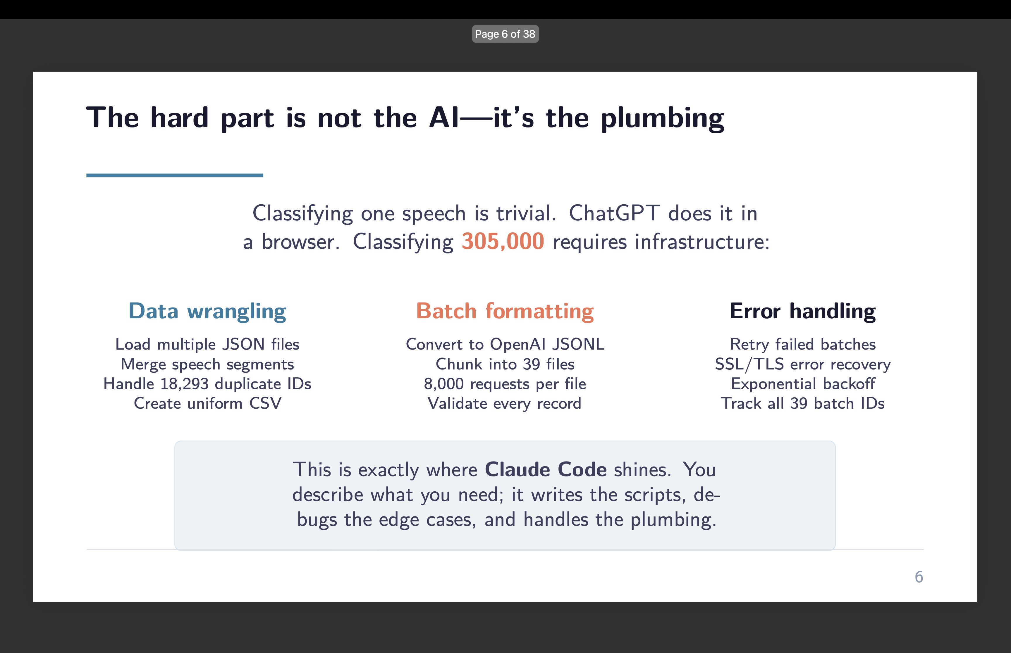
Jerry Seinfeld’s spouse as soon as mentioned that if she needs her children to eat greens, she hides them on a pizza. That’s been the working precept of this complete sequence. I’ve been replicating a PNAS paper — Card, et al on 140 years of congressional speeches and presidential communications about immigration — not as a result of the replication is the purpose, however as a result of the replication is the pizza. The greens are Claude Code and what it may possibly do whenever you level it at an actual analysis query.
My rivalry has been easy: you can’t be taught Claude Code by way of Claude Code alone. You’ll want to see it helping within the pursuit of one thing you already wished to do. Which is why this has been two issues directly from the beginning. First, an indication of what’s potential when an AI coding agent builds and runs your pipeline. Second, an precise analysis undertaking — one the place the LLM reclassification of 285,000 speeches turned up issues I didn’t anticipate finding.
And this sequence is about that. I exploit Claude Code on the service of analysis duties as a way to see it being finished by first following a analysis undertaking. That is how I’m “sneaking veggies onto the pizza” so to talk — by making this sequence in regards to the analysis use instances, not Claude Code itself, my hope is that you just see how you should utilize Claude Code for analysis too.
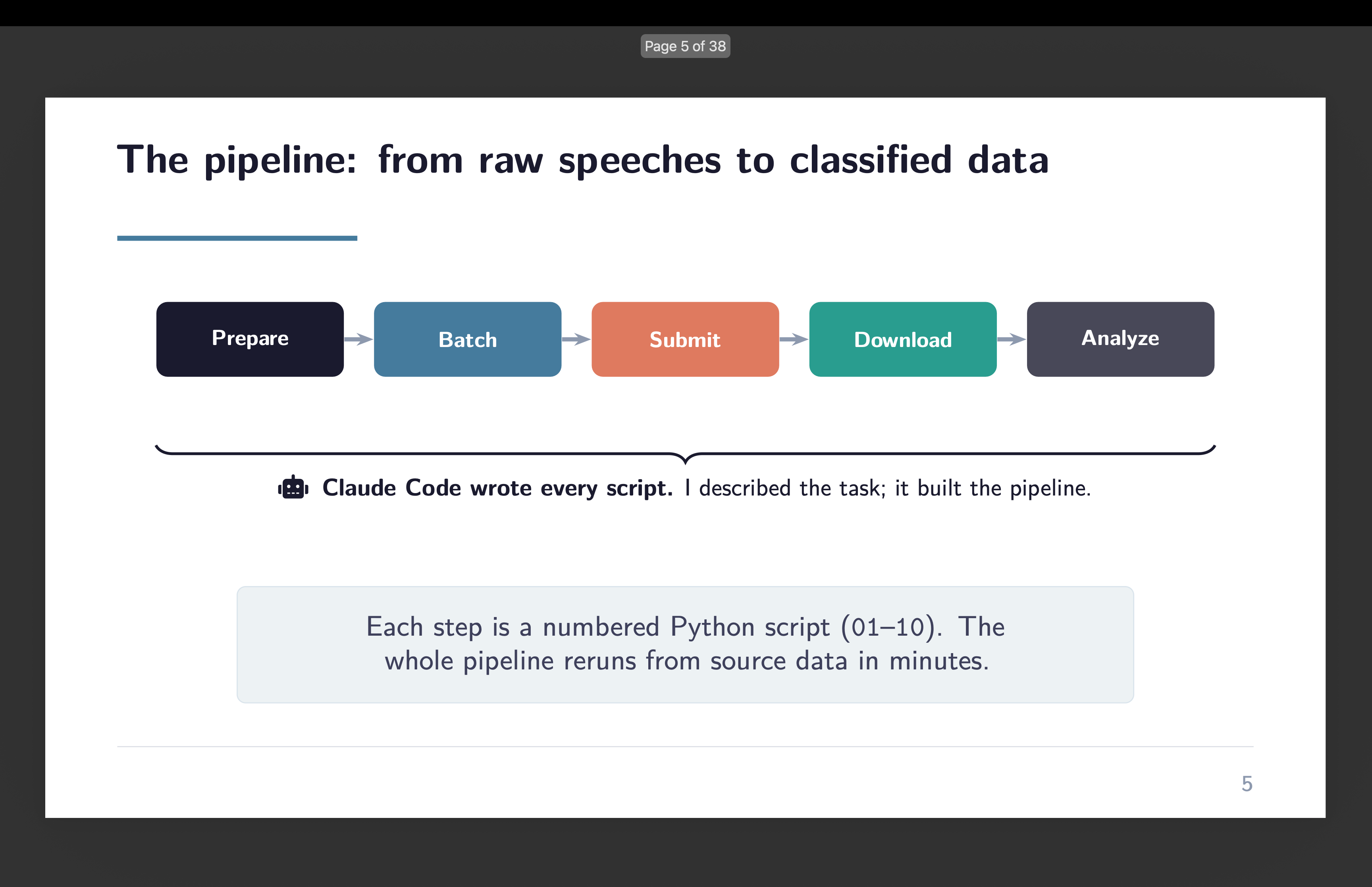
Within the first two components of this sequence, we constructed a pipeline utilizing Claude Code and OpenAI’s Batch API to reclassify each speech within the Card et al. dataset. The unique paper used a fine-tuned RoBERTa mannequin. Round 7 college students at Princeton rated 7500 speeches which have been then used with RoBERTa to foretell a pair hundred thousand extra.
However we used gpt-4o-mini at zero temperature, zero-shot, no coaching information. The entire value for the unique submission was eleven {dollars}. The entire time was about two and a half hours of computation, most of it ready on the Batch API. And after I redid it a second time, it was simply one other $11 and one other couple hours. Making the entire value of all this round $22 and roughly a day’s quantity of labor.
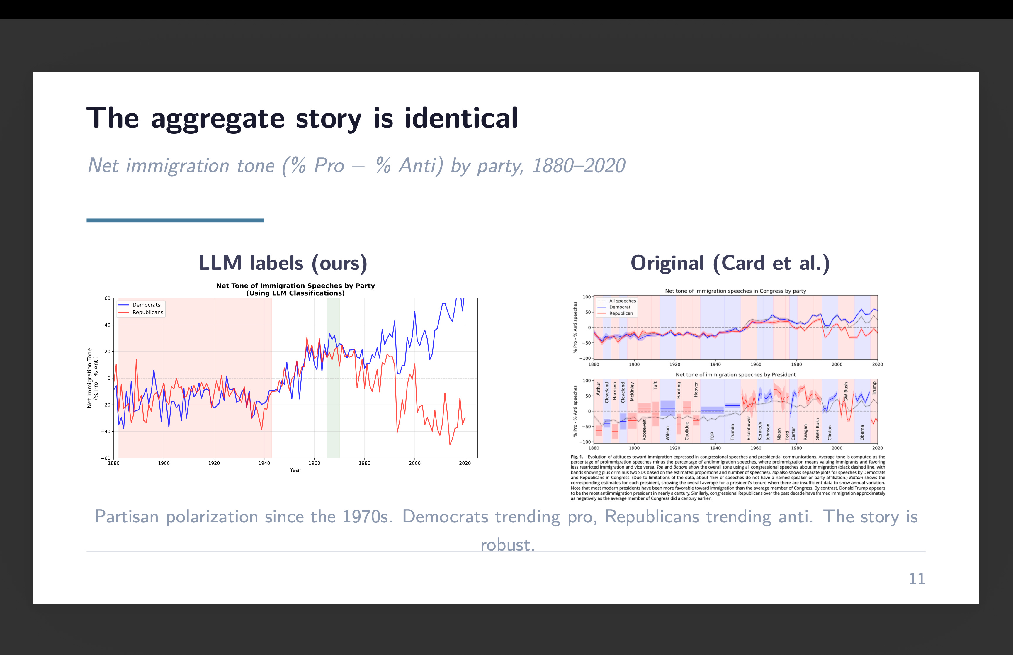
The headline outcome was 69% settlement with the unique classifications. The place the 2 fashions disagreed, the LLM overwhelmingly pulled towards impartial — as if it had the next threshold for calling one thing definitively pro- or anti-immigration. However right here’s the factor that made it publishable slightly than simply fascinating: the combination time sequence was just about equivalent. Decade by decade, the web tone of congressional immigration speeches tracked the identical trajectory no matter which mannequin did the classifying. The disagreements cancelled out as a result of they have been roughly symmetric.
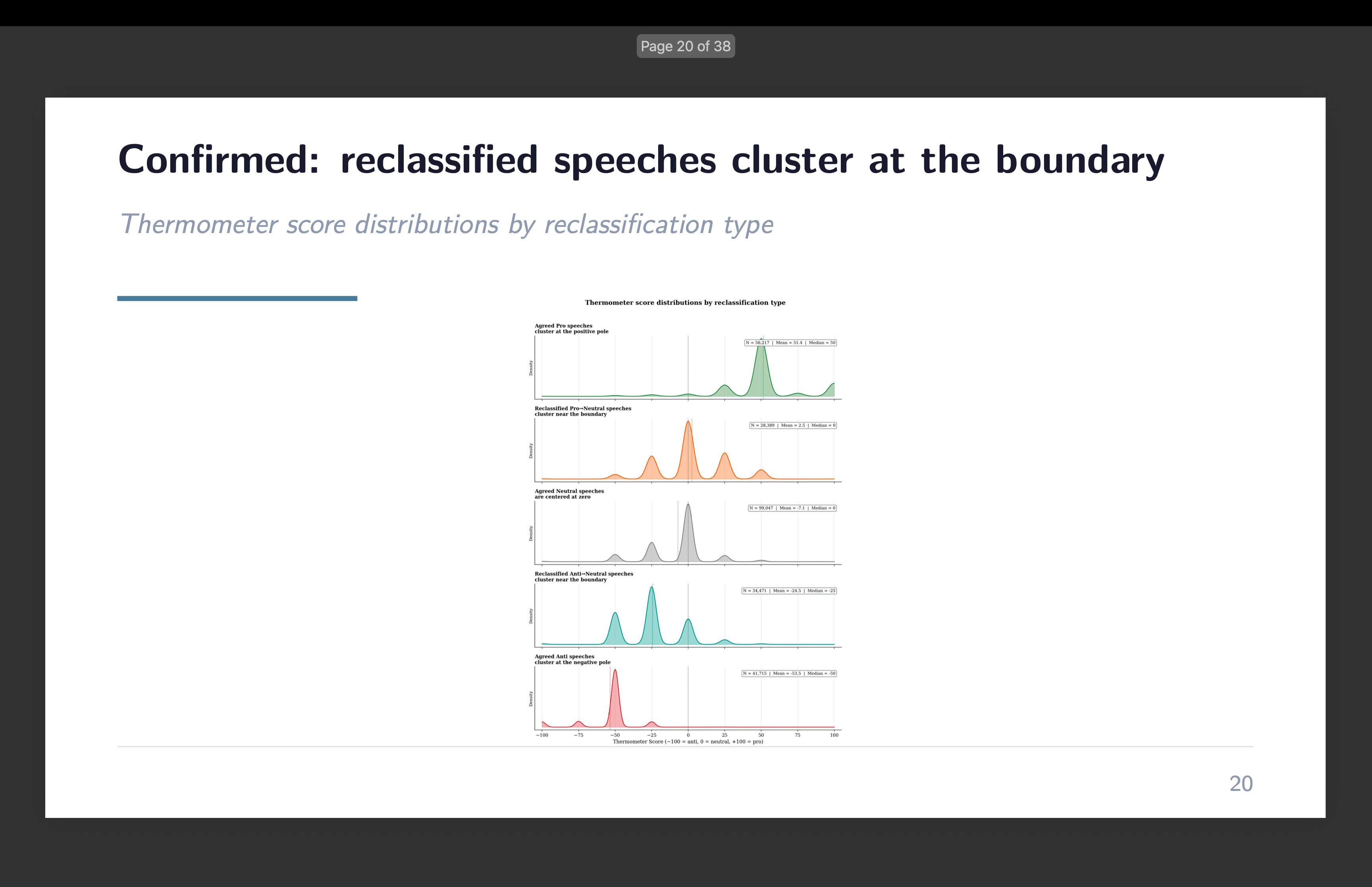
For the second submission, we wished to go deeper. As an alternative of simply asking the LLM for a label — professional, anti, or impartial — we requested it for a steady rating. A thermometer. Price every speech from -100 (strongly anti-immigration) to +100 (strongly pro-immigration). The thought was easy: if reclassified speeches actually are marginal instances, they need to cluster close to zero on the thermometer. And if the LLM is doing one thing essentially completely different from RoBERTa, the thermometer would expose it.
It labored. Speeches the place each fashions agreed on “anti” averaged round -54. Speeches each known as “professional” averaged round +48. And the reclassified speeches — those the LLM moved from the unique label to impartial — clustered nearer to zero, with technique of -25 and +2.5 respectively. The boundary instances behaved like boundary instances.
However one thing else confirmed up within the information. One thing I wasn’t searching for.
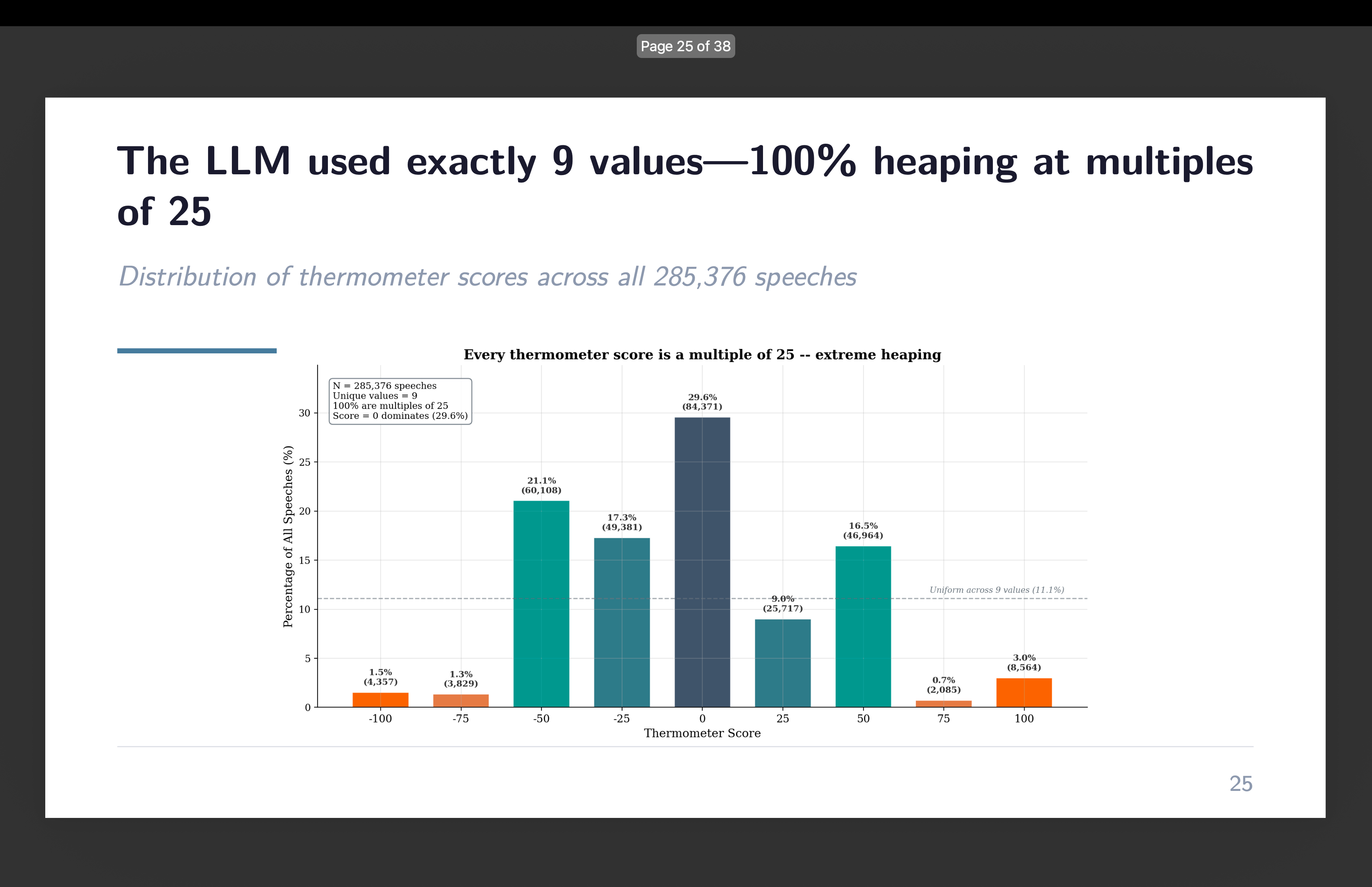
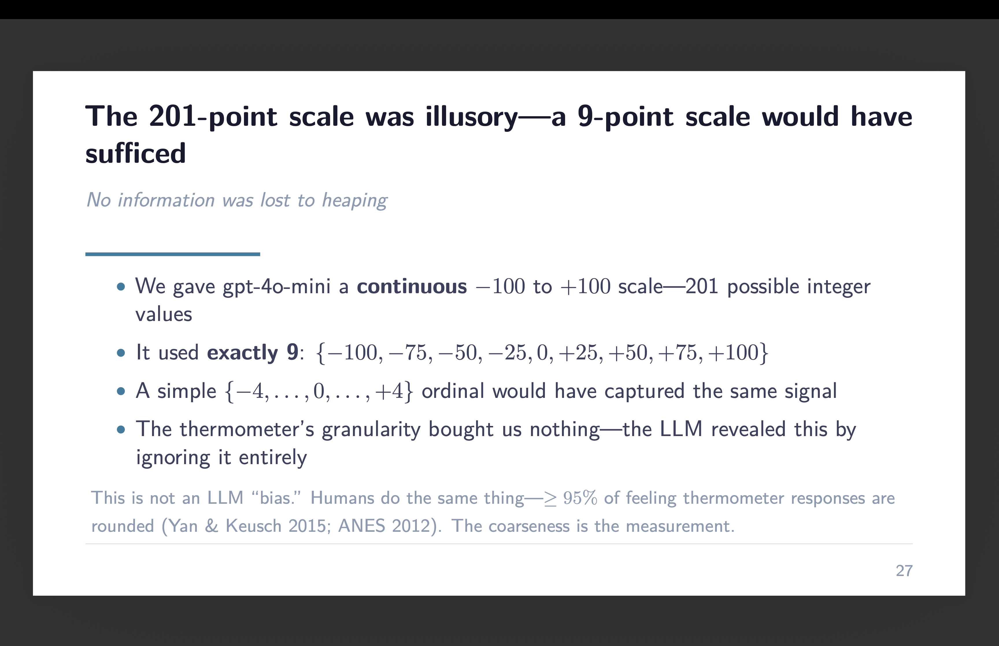
I gave gpt-4o-mini a steady scale. 200 and one potential integer values from -100 to +100. And it used 9 of them.
Each single thermometer rating — all 285,376 of them — landed on a a number of of 25. The values -100, -75, -50, -25, 0, +25, +50, +75, +100. That’s it. Not a single -30. Not one +42. Not a +17 wherever in a 3rd of 1,000,000 speeches. The mannequin spontaneously transformed a steady scale right into a 9-point ordinal.
After I noticed this, I ended the session. As a result of I acknowledged it. I had taught (my deck) about this simply yesterday mockingly in my Gov 51 class right here at Harvard.
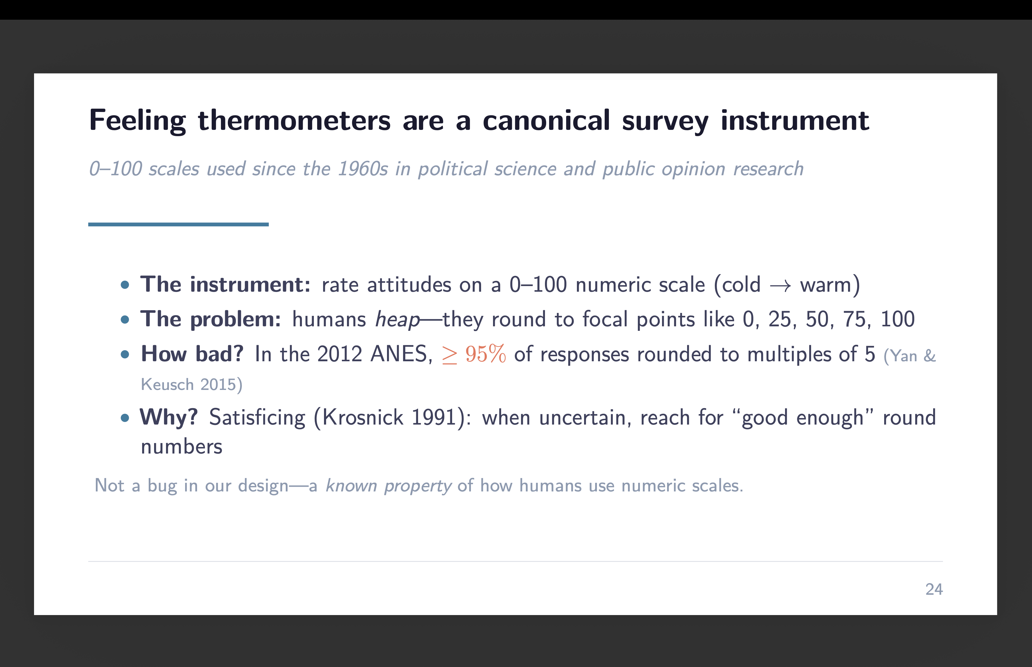
Feeling thermometers have been utilized in survey analysis because the Sixties. The American Nationwide Election Research use them. Political scientists use them to measure attitudes towards candidates, events, teams. You give somebody a scale from 0 to 100 and ask them to price how warmly they really feel about one thing. The instrument is in every single place.
And the instrument has a well-documented drawback: people heap. They spherical to focal factors. Within the 2012 ANES, at the least 95% of feeling thermometer responses have been rounded to multiples of 5. The modal responses are all the time 0, 50, and 100. Folks don’t use the total vary. They satisfice — a time period from Herbert Simon by the use of Jon Krosnick’s satisficing idea of survey response. Whenever you’re unsure about the place you fall on a 101-point scale, you attain for the closest spherical quantity that feels shut sufficient.
That is so well-known that it turned a part of a fraud detection case. The day earlier than I observed the heaping in our information, I’d been instructing Broockman, Kalla, and Aronow’s “irregularities” paper — the one which documented issues with the LaCour and Inexperienced research in Science. A part of their proof that LaCour’s information was fabricated concerned thermometer scores. The unique CCAP survey information confirmed the anticipated heaping sample — massive spikes at 0, 50, 100. LaCour’s management group information didn’t. It appeared he’d injected small random noise from a standard distribution, which smoothed the heaps away. The heaping was so anticipated that its absence was a purple flag.
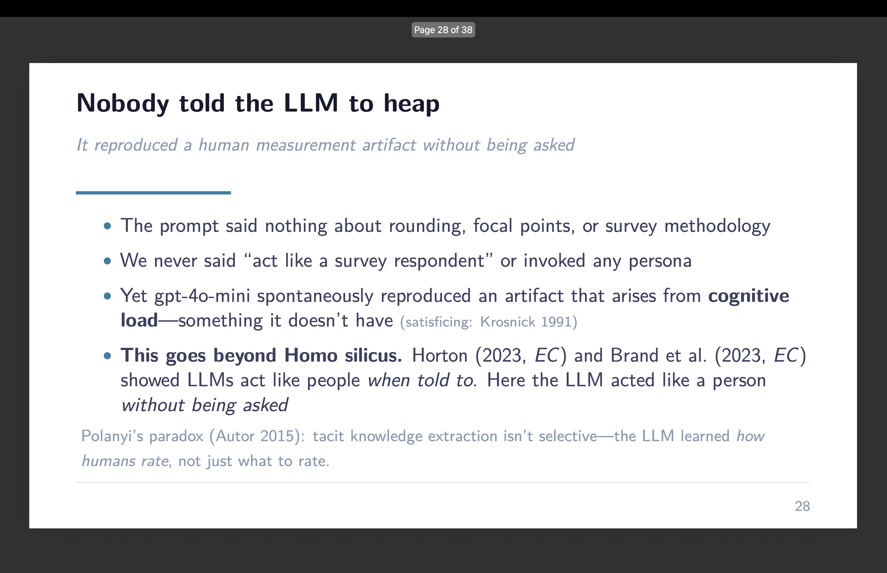
Right here’s what stops me. The unique Card et al. paper didn’t use a thermometer. RoBERTa doesn’t produce scores on a sense thermometer scale. I invented the -100 to +100 framing for this undertaking. The immediate mentioned nothing about survey methodology, nothing about rounding, nothing about appearing like a survey respondent. I gave gpt-4o-mini a classification activity with a steady output area and it voluntarily compressed that area in precisely the way in which a human survey respondent would.
The LLM doesn’t have cognitive load. It doesn’t get drained. It doesn’t expertise the uncertainty that makes people attain for spherical numbers. Satisficing is a idea about bounded rationality — in regards to the hole between what you’d do with infinite processing capability and what you truly do with a organic mind that has different issues to fret about. The LLM has no such hole. And but it heaped.
This goes past what others have documented. John Horton’s “Homo Silicus” work confirmed that LLMs reproduce outcomes from basic financial experiments — they exhibit equity norms, established order bias, the type of habits we anticipate from human topics — at roughly a greenback per experiment. Model, Israeli, and Ngwe confirmed that GPT reveals downward-sloping demand curves, constant willingness-to-pay, state dependence — the constructing blocks of rational client habits. Each of these findings are hanging. However in each instances, the researchers informed the LLM to behave like an individual. They gave it a persona. They mentioned “you’re a participant on this experiment” or “you’re a client evaluating this product.”
I didn’t inform gpt-4o-mini to behave like something. I informed it to categorise speeches. And it categorized them — accurately, usefully, in a manner that replicates the unique paper’s combination findings. However it additionally, with out being requested, reproduced a measurement artifact that arises from human cognitive limitations it doesn’t possess.
Autor’s perception about LLMs is that they seem to have cracked this paradox. They extract tacit information from coaching information. They will do issues nobody ever wrote guidelines for as a result of they discovered from the gathered output of people doing these issues.
However right here’s what the heaping suggests: the extraction isn’t selective. When the LLM discovered consider political speech on a numeric scale, it didn’t simply be taught what to price every speech. It discovered how people price. It absorbed the content material information and the measurement noise collectively, as a bundle. The heaping, the rounding, the focal-point heuristics — these got here alongside for the journey. No one educated gpt-4o-mini on survey methodology. No one labeled a dataset with “that is what satisficing seems like.” The mannequin discovered it the way in which people be taught it: implicitly, from publicity, with out anybody pointing it out.
I believe that is the type of tacit information Autor has in thoughts. The issues nobody ever informed anybody to do, as a result of nobody knew they have been doing them.
There was additionally a sensible query hanging over the entire undertaking: does any of this depend upon the truth that we had three classes? Professional, anti, and impartial type a pure spectrum with a middle that may take in errors. Possibly the symmetric cancellation solely works as a result of impartial sits between the opposite two.
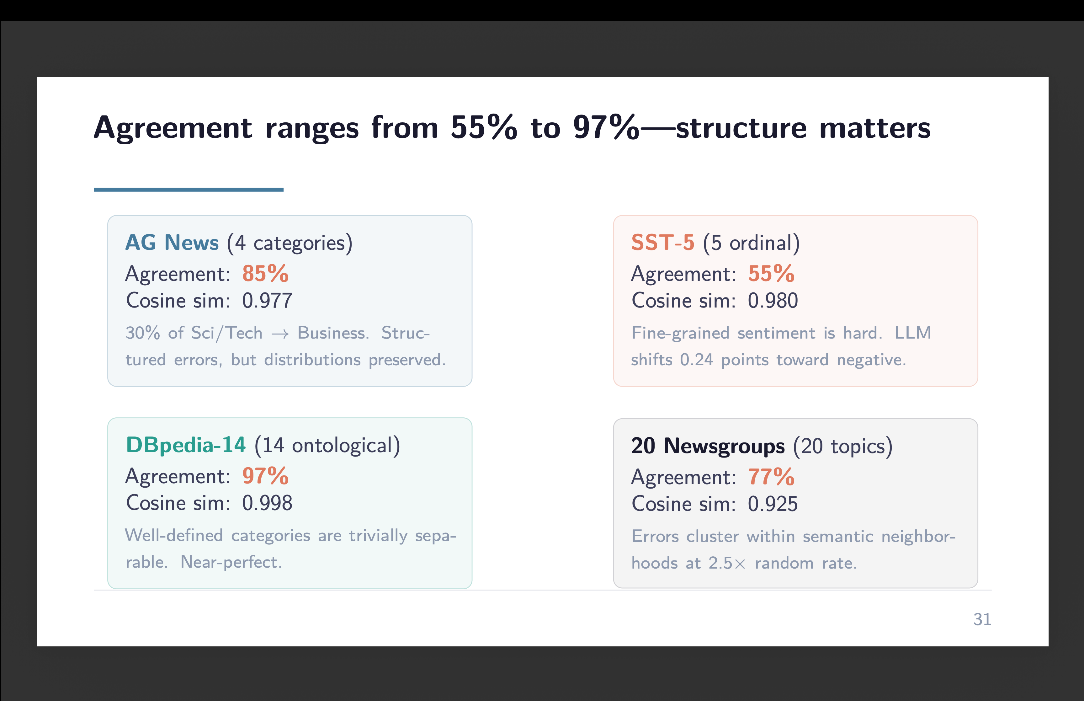
So we examined 4 benchmark datasets: AG Information (4 classes, no ordering), SST-5 (5-level sentiment with a middle), DBpedia-14 (14 ontological classes), and 20 Newsgroups (20 unordered subjects). Similar methodology — zero-shot gpt-4o-mini, temperature zero, Batch API. Complete value for all 4: a greenback twenty-six.
Settlement ranged from 55% on 20 Newsgroups to 97% on DBpedia-14. The mechanism wasn’t tripartite construction. It was class separability — how distinct the classes are from one another. When the classes are semantically crisp (firm vs. faculty vs. artist in DBpedia), the LLM nails it. After they’re fuzzy and overlapping (distinguishing speak.politics.weapons from speak.politics.misc in Newsgroups), it struggles. The immigration outcome generalizes, however not as a result of three classes are particular. It generalizes as a result of the classes occur to be fairly separable.
Another factor. Whereas we have been doing this work, Asirvatham, Mokski, and Shleifer launched an NBER working paper known as “GPT as a Measurement Instrument.” They current a software program bundle — GABRIEL — that makes use of GPT to quantify attributes in qualitative information. One among their check instances is congressional remarks. The paper supplies impartial proof that GPT-based classification can match or exceed human-annotated approaches for the type of political textual content evaluation we’ve been doing.
I point out this to not declare precedence however to notice convergence. A number of teams are arriving on the identical place from completely different instructions. The LLM isn’t only a classifier. It’s a measurement instrument. And like all measurement devices, it has properties — together with properties no one designed into it.
I began this sequence wanting to indicate folks what Claude Code can do. I nonetheless suppose one of the best ways to be taught it’s to look at it work on one thing actual. However the one thing actual saved producing surprises. The 69% settlement that doesn’t matter as a result of the disagreements cancel. The thermometer scores that cluster on the boundary. And now this — a measurement artifact that no one requested for, that no one programmed, that emerges from the identical tacit information that makes the classification work within the first place.
A 9-point scale hidden inside a 201-point scale. The LLM measures like a human, right down to the errors. And I don’t suppose it is aware of it’s doing it any greater than we do.
Effectively, that’s the top of this replication/extension of the PNAS paper. I wished folks to see with their very own eyes the usage of Claude Code to do classification of texts utilizing gpt-4o-mini at OpenAI. It’s not an easy factor. Listed here are two slides about it:
And in order that’s finished. I hope that the video stroll throughs, and the reasons, in addition to the decks (like this remaining one) have been useful for a few of you on the fence about utilizing Claude Code. Not solely do I believe that it’s a useful productiveness enhancing instrument — to be trustworthy, I believe it’s unavoidable. It’s most likely on par with the transfer from utilizing punch playing cards for empirical work to what we have now now. Possibly even moreso. However having supplies that enable you to get there I believe is for many individuals actually important as a lot of the materials till not too long ago was by engineers for engineers, and admittedly, I believe Claude Code could also be placing these particular duties into pure automation which means even these explainers may fade.
However now I’ve to determine what I’m going to do with these findings! So we’ll see if I can work out a paper out of all this bumbling round that you just noticed. Undecided. I both am staring proper at a small contribution or I’m seeing a mirage and nothing is there, however I’m going to suppose on that subsequent. I’m open to ideas! Have an incredible weekend! Keep hydrated because the flu could also be going round.
AI is evolving quickly, and software program engineers not must memorize syntax. Nonetheless, considering like an architect and understanding the know-how that permits techniques to run securely at scale is turning into more and more useful.
I additionally wish to replicate on being in my function a yr now as an AI Options Engineer at Cisco. I work with clients each day throughout totally different verticals — healthcare, monetary providers, manufacturing, legislation corporations, and they’re all making an attempt to reply largely the identical set of questions:
What’s our AI technique?
What use instances truly match our knowledge?
Cloud vs. on-prem vs. hybrid?
How a lot will it value — not simply as we speak, however at scale?
How can we safe it?
These are the true sensible constraints that present up instantly when you attempt to operationalize AI past a POC.
Lately, we added a Cisco UCS C845A to one among our labs. It has 2x NVIDIA RTX PRO 6000 Blackwell GPUs, 3.1TB NVMe, ~127 allocatable CPU cores, and 754GB RAM. I made a decision to construct a shared inner platform on high of it — giving groups a constant, self-service surroundings to run experiments, validate concepts, and construct hands-on GPU expertise.
I deployed the platform as a Single Node OpenShift (SNO) cluster and layered a multi-tenant GPUaaS expertise on high. Customers reserve capability by way of a calendar UI, and the system provisions an remoted ML surroundings prebuilt with PyTorch/CUDA, JupyterLab, VS Code, and extra. Inside that surroundings, customers can run on-demand inference, iterate on mannequin coaching and fine-tuning, and prototype manufacturing grade microservices.
This put up walks by way of the structure — how scheduling selections are made, how tenants are remoted, and the way the platform manages itself. The selections that went into this lab platform are the identical ones any group faces after they’re critical about AI in manufacturing.
That is the inspiration for enterprise AI at scale. Multi-agent architectures, self-service experimentation, safe multi-tenancy, cost-predictable GPU compute, all of it begins with getting the platform layer proper.
Excessive degree platform structure diagram. Picture created by writer.
Preliminary Setup
Earlier than there’s a platform, there’s a naked steel server and a clean display.
Bootstrapping the Node
The node ships with no working system. Whenever you energy it on you’re dropped right into a UEFI shell. For OpenShift, set up usually begins within the Pink Hat Hybrid Cloud Console through the Assisted Installer. The Assisted Installer handles cluster configuration by way of a guided setup stream, and as soon as full, generates a discovery ISO — a bootable RHEL CoreOS picture preconfigured in your surroundings. Map the ISO to the server as digital media by way of the Cisco IMC, set boot order, and energy on. The node will telephone house to the console, and you may kick off the set up course of. The node writes RHCOS to NVMe and bootstraps. Inside a number of hours you might have a working cluster.
This workflow assumes web connectivity, pulling photos from Pink Hat’s registries throughout set up. That’s not at all times an possibility. Lots of the clients I work with function in air-gapped environments the place nothing touches the general public web. The method there’s totally different: generate ignition configs regionally, obtain the OpenShift launch photos and operator bundles forward of time, mirror the whole lot into a neighborhood Quay registry, and level the set up at that. Each paths get you to the identical place. The assisted set up is far simpler. The air-gapped path is what manufacturing appears like in regulated industries.
Configuring GPUs with the NVIDIA GPU Operator
As soon as the GPU Operator is put in (occurs robotically utilizing the assisted installer), I configured how the 2 RTX PRO 6000 Blackwell GPUs are offered to workloads by way of two ConfigMaps within the nvidia-gpu-operator namespace.
The primary — custom-mig-config — defines bodily partitioning. On this case it’s a combined technique, that means GPU 0 is partitioned into 4 1g.24gb MIG slices (~24GB devoted reminiscence every), GPU 1 stays complete for workloads that want the complete ~96GB. MIG partitioning is actual {hardware} isolation. You get devoted reminiscence, compute models, and L2 cache per slice. Workloads will see MIG situations as separate bodily units.
The second — device-plugin-config — configures time-slicing, which permits a number of pods to share the identical GPU or MIG slice by way of fast context switching. I set 4 replicas per complete GPU and a couple of per MIG slice. That is what permits working a number of inference containers facet by facet inside a single session.
Foundational Storage
The three.1TB NVMe is managed by the LVM Storage Operator (lvms-vg1 StorageClass). I created two PVCs as part of the preliminary provisioning course of — a quantity backing PostgreSQL and chronic storage for OpenShift’s inner picture registry.
With the OS put in, community stipulations met (DNS, IP allocation, all required A data) which isn’t lined on this article, GPUs partitioned, and storage provisioned, the cluster is prepared for the appliance layer.
System Structure
This leads us into the primary subject: the system structure. The platform separates into three planes — scheduling, management, and runtime, with the PostgreSQL database as the one supply of reality.
Within the platform administration namespace, there are 4 at all times on deployments:
Portal app: a single container working the React UI and FastAPI backend
Reconciler (controller): the management loop that repeatedly converges cluster state to match the database
PostgreSQL: persistent state for customers, reservations, tokens, and audit historical past
Cache daemon: a node-local service that pre-stages giant mannequin artifacts / inference engines so customers can begin shortly (pulling a 20GB vLLM picture over company proxy can take hours)
A fast notice on the event lifecycle, as a result of it’s straightforward to complicate delivery Kubernetes techniques. I write and take a look at code regionally, however the photos are constructed within the cluster utilizing OpenShift construct artifacts (BuildConfigs) and pushed to the inner registry. The deployments themselves simply level at these photos.
The primary time a element is launched, I apply the manifests to create the Deployment/Service/RBAC. After that, most modifications are simply constructing a brand new picture in-cluster, then set off a restart so the Deployment pulls the up to date picture and rolls ahead:
That is the person going through entry level. Customers see the useful resource pool — GPUs, CPU, reminiscence, they choose a time window, select their GPU allocation mode (extra on this later), and submit a reservation.
GPUs are costly {hardware} with an actual value per hour whether or not they’re in use or not. The reservation system treats calendar time and bodily capability as a mixed constraint. The identical method you’d e book a convention room, besides this room has 96GB of VRAM and prices significantly extra per hour.
Underneath the hood, the system queries overlapping reservations in opposition to pool capability utilizing advisory locks to forestall double reserving. Primarily it’s simply including up reserved capability and subtracting it from whole capability. Every reservation tracks by way of a lifecycle: APPROVED → ACTIVE → COMPLETED, with CANCELED and FAILED as terminal states.
The FastAPI server itself is deliberately skinny. It validates enter, persists the reservation, and returns. It by no means talks to the Kubernetes API.
The Management Aircraft
On the coronary heart of the platform is the controller. It’s Python based mostly and runs in a steady loop on a 30-second cadence. You’ll be able to consider it like a cron job when it comes to timing, however architecturally it’s a Kubernetes-style controller liable for driving the system towards a desired state.
The database holds the specified state (reservations with time home windows and useful resource necessities). The reconciler reads that state, compares it in opposition to what truly exists within the Kubernetes cluster, and converges the 2. There aren’t any concurrent API calls racing to mutate cluster state; only one deterministic loop making the minimal set of modifications wanted to succeed in the specified state. If the reconciler crashes, it restarts and continues precisely the place it left off, as a result of the supply of reality (desired state) stays intact within the database.
Every reconciliation cycle evaluates 4 considerations so as:
Cease expired or canceled classes and delete the namespace (which cascades cleanup of all assets inside it).
Restore failed classes and take away orphaned assets left behind by partially accomplished provisioning.
Begin eligible classes when their reservation window arrives — provision, configure, and hand the workspace to the person.
Keep the database by expiring previous tokens and imposing audit log retention.
Beginning a session is a multi-step provisioning sequence, and each step is idempotent, that means it’s designed to be safely re-run if interrupted halfway:
Controller in depth. Picture created by writer.
The reconciler is the solely element that talks to the Kubernetes API.
Rubbish assortment can also be baked into the identical loop. At a slower cadence (~5 minutes), the reconciler sweeps for cross namespace orphans equivalent to stale RBAC bindings, leftover OpenShift safety context entries, namespaces caught in terminating, or namespaces that exist within the cluster however haven’t any matching database document.
The design assumption all through is that failure is regular. For instance, we had an influence provide failure on the node that took the cluster down mid-session and when it got here again, the reconciler resumed its loop, detected the state discrepancies, and self-healed with out guide intervention.
The Runtime Aircraft
When a reservation window begins, the person opens a browser and lands in a full VS Code workspace (code-server) pre-loaded with the complete AI/ML stack, and kubectl entry inside their session namespace.
Workspace screenshot. Picture taken by writer.
Standard inference engines equivalent to vLLM, Ollama, TGI, and Triton are already cached on the node, so deploying a mannequin server is a one-liner that begins in seconds. There’s 600GB of persistent NVMe backed storage allotted to the session, together with a 20GB house listing for notebooks and scripts, and a 300GB mannequin cache.
Every session is a totally remoted Kubernetes namespace, its personal blast radius boundary with devoted assets and 0 visibility into every other tenant’s surroundings. The reconciler provisions namespace scoped RBAC granting full admin powers inside that boundary, enabling customers to create and delete pods, deployments, providers, routes, secrets and techniques — regardless of the workload requires. However there’s no cluster degree entry. Customers can learn their very own ResourceQuota to see their remaining price range, however they’ll’t modify it.
ResourceQuota enforces a tough ceiling on the whole lot. A runaway coaching job can’t OOM the node. A rogue container can’t fill the NVMe. LimitRange injects sane defaults into each container robotically, so customers can kubectl run with out specifying useful resource requests. There’s a proxy ConfigMap injected into the namespace so person deployed containers get company community egress with out guide configuration.
Customers deploy what they need — inference servers, databases, {custom} providers, and the platform handles the guardrails.
When the reservation window ends, the reconciler deletes the namespace and the whole lot inside it.
GPU Scheduling
Node multi-tenancy diagram. Picture created by writer.
Now the enjoyable half — GPU scheduling and truly working hardware-accelerated workloads in a multi-tenant surroundings.
MIG & Time-slicing
We lined the MIG configuration within the preliminary setup, but it surely’s price revisiting from a scheduling perspective. GPU 0 is partitioned into 4 1g.24gb MIG slices — every with ~24GB of devoted reminiscence, sufficient for many 7B–14B parameter fashions. GPU 1 stays complete for workloads that want the complete ~96GB VRAM for mannequin coaching, full-precision inference on 70B+ fashions, or something that merely doesn’t slot in a slice.
The reservation system tracks these as distinct useful resource varieties. Customers e book both nvidia.com/gpu (complete) or nvidia.com/mig-1g.24gb (as much as 4 slices). The ResourceQuota for every session exhausting denies the alternative sort. If you happen to reserved a MIG slice, you bodily can’t request an entire GPU, even when one is sitting idle. In a combined MIG surroundings, letting a session by chance devour the flawed useful resource sort would break the capability math for each different reservation on the calendar.
Time-slicing permits a number of pods to share the identical bodily GPU or MIG slice by way of fast context switching. The NVIDIA system plugin advertises N “digital” GPUs per bodily system.
In our configuration, 1 complete GPU seems as 4 schedulable assets. Every MIG slice seems as 2.
What which means is a person reserves one bodily GPU and may run as much as 4 concurrent GPU-accelerated containers inside their session — a vLLM occasion serving gpt-oss, an Ollama occasion with Mistral, a TGI server working a reranker, and a {custom} service orchestrating throughout all three.
Two Allocation Modes
At reservation time, customers select how their GPU price range is initially distributed between the workspace and person deployed containers.
Interactive ML — The workspace pod will get a GPU (or MIG slice) connected instantly. The person opens Jupyter, imports PyTorch, and has quick CUDA entry for coaching, fine-tuning, or debugging. Further GPU pods can nonetheless be spawned through time-slicing, however the workspace is consuming one of many digital slots.
Inference Containers — The workspace is light-weight with no GPU connected. All time-sliced capability is offered for person deployed containers. With an entire GPU reservation, that’s 4 full slots for inference workloads.
There’s a actual throughput tradeoff with time-slicing, workloads share VRAM and compute bandwidth. For growth, testing, and validating multi-service architectures, which is precisely what this platform is for, it’s the correct trade-off. For manufacturing latency delicate inference the place each millisecond of p99 issues, you’d use devoted slices 1:1 or complete GPUs.
GPU “Tokenomics”
One of many first questions within the introduction was: How a lot will it value — not simply as we speak, however at scale? To reply that, it’s a must to begin with what the workload truly appears like in manufacturing.
What Actual Deployments Look Like
Once I work with clients on their inference structure, no person is working a single mannequin behind a single endpoint. The sample that retains rising is a fleet of fashions sized to the duty. You have got a 7B parameter mannequin dealing with easy classification and extraction, runs comfortably on a MIG slice. A 14B mannequin doing summarization and normal goal chat. A 70B mannequin for complicated reasoning and multi-step duties, and perhaps a 400B mannequin for the toughest issues the place high quality is non-negotiable. Requests get routed to the suitable mannequin based mostly on complexity, latency necessities, or value constraints. You’re not paying 70B-class compute for a activity a 7B can deal with.
In multi-agent techniques, this will get extra attention-grabbing. Brokers subscribe to a message bus and sit idle till known as upon — a pub-sub sample the place context is shared to the agent at invocation time and the pod is already heat. There’s no chilly begin penalty as a result of the mannequin is loaded and the container is working. An orchestrator agent evaluates the inbound request, routes it to a specialist agent (retrieval, code era, summarization, validation), collects the outcomes, and synthesizes a response. 4 or 5 fashions collaborating on a single person request, every working in its personal container inside the identical namespace, speaking over the inner Kubernetes community.
Community insurance policies add one other dimension. Not each agent ought to have entry to each instrument. Your retrieval agent can speak to the vector database. Your code execution agent can attain a sandboxed runtime. However the summarization agent has no enterprise touching both, it receives context from the orchestrator and returns textual content. Community insurance policies implement these boundaries on the cluster degree, so instrument entry is managed by infrastructure, not utility logic.
That is the workload profile the platform was designed for. MIG slicing allows you to proper measurement GPU allocation per mannequin, a 7B doesn’t want 96GB of VRAM. Time-slicing lets a number of brokers share the identical bodily system. Namespace isolation retains tenants separated whereas brokers inside a session talk freely. The structure instantly helps these patterns.
Quantifying It
To maneuver from structure to enterprise case, I developed a tokenomics framework that reduces infrastructure value to a single comparable unit: value per million tokens. Every token carries its amortized share of {hardware} capital (together with workload combine and redundancy), upkeep, energy, and cooling. The numerator is your whole annual value. The denominator is what number of tokens you truly course of, which is fully a perform of utilization.
Utilization is probably the most highly effective lever on per-token value. It doesn’t cut back what you spend, the {hardware} and energy payments are mounted. What it does is unfold these mounted prices throughout extra processed tokens. A platform working at 80% utilization produces tokens at practically half the unit value of 1 at 40%. Identical infrastructure, dramatically totally different economics. That is why the reservation system, MIG partitioning, and time-slicing matter past UX — they exist to maintain costly GPUs processing tokens throughout as many obtainable hours as attainable.
As a result of the framework is algebraic, you may also remedy within the different path. Given a identified token demand and a price range, remedy for the infrastructure required and instantly see whether or not you’re over-provisioned (burning cash on idle GPUs), under-provisioned (queuing requests and degrading latency), or right-sized.
For the cloud comparability, suppliers have already baked their utilization, redundancy, and overhead into per-token API pricing. The query turns into: at what utilization does your on-prem unit value drop under that charge? For constant enterprise GPU demand, the sort of steady-state inference visitors these multi-agent architectures generate, on-prem wins.
Cloud token prices in multi-agent environments scale parabolically.
Nonetheless, for testing, demos, and POCs, cloud is cheaper.
Engineering groups typically must justify spend to finance with clear, defensible numbers. The tokenomics framework bridges that hole.
Conclusion
Firstly of this put up I listed the questions I hear from clients continuously — AI technique, use-cases, cloud vs. on-prem, value, safety. All of them finally require the identical factor: a platform layer that may schedule GPU assets, isolate tenants, and provides groups a self-service path from experiment to manufacturing with out ready on infrastructure.
That’s what this put up walked by way of. Not a product and never a managed service, however an structure constructed on Kubernetes, PostgreSQL, Python, and the NVIDIA GPU Operator — working on a single Cisco UCS C845A with two NVIDIA RTX PRO 6000 Blackwell GPUs in our lab. It’s a sensible start line that addresses scheduling, multi-tenancy, value modeling, and the day-2 operational realities of retaining GPU infrastructure dependable.
This isn’t as intimidating because it appears. The tooling is mature, and you may assemble a cloud-like workflow with acquainted constructing blocks: reserve GPU capability from a browser, drop into a totally loaded ML workspace, and spin up inference providers in seconds. The distinction is the place it runs — on infrastructure you personal, below your operational management, with knowledge that by no means leaves your 4 partitions. In apply, the barrier to entry is usually decrease than leaders count on.
Scale this to a number of Cisco AI Pods and the scheduling airplane, reconciler sample, and isolation mannequin carry over instantly. The inspiration is similar.
If you happen to’re working by way of these identical selections — tips on how to schedule GPUs, tips on how to isolate tenants, tips on how to construct the enterprise case for on-prem AI infrastructure, I’d welcome the dialog.
I’m an AI Options Engineer at Cisco, specializing in enterprise AI infrastructure. Attain out at [email protected].
It begins quietly, as many tales do, in a small rural city the place the horizon appears impossibly broad. The city planning fee gathers in a modest room, the air thick with the scent of burnt espresso and aged carpet, to listen to that their city will quickly win the fashionable financial system: 10 new knowledge facilities throughout the city’s boundaries. Not only one or two, however 10. The PowerPoint displays shine with guarantees: development jobs, some everlasting positions, “group funding,” and a brand new tax base that can “remodel the area.”
Positive, there might be jobs. However not the roles that rebuild a city’s soul. Information facilities don’t make use of hundreds as soon as they’re up; they make use of dozens, generally fewer, relying on how automated the operation is. The actual influence isn’t folks—it’s energy, land, transmission capability, and water. Whenever you drop 10 large services right into a small grid, demand spikes don’t simply occur contained in the fence line. They ripple outward. Utilities should improve substations, reinforce transmission strains, procure new-generation tools, and finance these investments. Guess who finally ends up paying a significant portion of that over time? Native ratepayers, in a single type or one other, will face larger payments or the quiet deferral of different infrastructure work.
Water is commonly the second shoe to drop. Even when operators insist they’re “water environment friendly,” cooling is cooling, and cooling at scale isn’t free. Some services will use evaporative techniques; some will use closed-loop techniques; some will promise innovation that seems spectacular in a press launch. In the meantime, the city’s farmers now watch the aquifer ranges and the climate forecast with equal nervousness, besides now they’re competing with an trade whose thirst is measured in engineering diagrams, not drought tales.
What could possibly be treacherous about abstract statistics?
The well-known cat chubby examine (X. et al., 2019) confirmed that as of Could 1st, 2019, 32 of 101 home cats held in Y., a comfy Bavarian village, had been chubby. Regardless that I’d be curious to know if my aunt G.’s cat (a cheerful resident of that village) has been fed too many treats and has collected some extra kilos, the examine outcomes don’t inform.
Then, six months later, out comes a brand new examine, bold to earn scientific fame. The authors report that of 100 cats residing in Y., 50 are striped, 31 are black, and the remainder are white; the 31 black ones are all chubby. Now, I occur to know that, with one exception, no new cats joined the neighborhood, and no cats left. However, my aunt moved away to a retirement residence, chosen in fact for the likelihood to carry one’s cat.
What have I simply discovered? My aunt’s cat is chubby. (Or was, a minimum of, earlier than they moved to the retirement residence.)
Regardless that not one of the research reported something however abstract statistics, I used to be in a position to infer individual-level details by connecting each research and including in one other piece of knowledge I had entry to.
In actuality, mechanisms just like the above – technically known as linkage – have been proven to result in privateness breaches many instances, thus defeating the aim of database anonymization seen as a panacea in lots of organizations. A extra promising different is obtainable by the idea of differential privateness.
Differential Privateness
In differential privateness (DP)(Dwork et al. 2006), privateness shouldn’t be a property of what’s within the database; it’s a property of how question outcomes are delivered.
Intuitively paraphrasing outcomes from a site the place outcomes are communicated as theorems and proofs (Dwork 2006)(Dwork and Roth 2014), the one achievable (in a lossy however quantifiable approach) goal is that from queries to a database, nothing extra ought to be discovered about a person in that database than in the event that they hadn’t been in there in any respect.(Wooden et al. 2018)
What this assertion does is warning towards overly excessive expectations: Even when question outcomes are reported in a DP approach (we’ll see how that goes in a second), they allow some probabilistic inferences about people within the respective inhabitants. (In any other case, why conduct research in any respect.)
So how is DP being achieved? The primary ingredient is noise added to the outcomes of a question. Within the above cat instance, as an alternative of actual numbers we’d report approximate ones: “Of ~ 100 cats residing in Y, about 30 are chubby….” If that is performed for each of the above research, no inference might be potential about aunt G.’s cat.
Even with random noise added to question outcomes although, solutions to repeated queries will leak data. So in actuality, there’s a privateness price range that may be tracked, and could also be used up in the midst of consecutive queries.
That is mirrored within the formal definition of DP. The thought is that queries to 2 databases differing in at most one aspect ought to give principally the identical end result. Put formally (Dwork 2006):
A randomized perform (mathcal{Okay}) offers (epsilon) -differential privateness if for all information units D1 and D2 differing on at most one aspect, and all (S subseteq Vary(Okay)),
(Pr[mathcal{K}(D1)in S] leq exp(epsilon) × Pr[K(D2) in S])
This (epsilon) -differential privateness is additive: If one question is (epsilon)-DP at a price of 0.01, and one other one at 0.03, collectively they are going to be 0.04 (epsilon)-differentially personal.
If (epsilon)-DP is to be achieved through including noise, how precisely ought to this be performed? Right here, a number of mechanisms exist; the fundamental, intuitively believable precept although is that the quantity of noise ought to be calibrated to the goal perform’s sensitivity, outlined as the utmost (ell 1) norm of the distinction of perform values computed on all pairs of datasets differing in a single instance (Dwork 2006):
(Delta f = max_{D1,D2} _1)
Thus far, we’ve been speaking about databases and datasets. How does this apply to machine and/or deep studying?
TensorFlow Privateness
Making use of DP to deep studying, we wish a mannequin’s parameters to wind up “basically the identical” whether or not educated on a dataset together with that cute little kitty or not. TensorFlow (TF) Privateness (Abadi et al. 2016), a library constructed on high of TF, makes it straightforward on customers so as to add privateness ensures to their fashions – straightforward, that’s, from a technical viewpoint. (As with life total, the onerous selections on how a lot of an asset we ought to be reaching for, and commerce off one asset (right here: privateness) with one other (right here: mannequin efficiency), stay to be taken by every of us ourselves.)
Concretely, about all we’ve got to do is alternate the optimizer we had been utilizing towards one offered by TF Privateness. TF Privateness optimizers wrap the unique TF ones, including two actions:
To honor the precept that every particular person coaching instance ought to have simply reasonable affect on optimization, gradients are clipped (to a level specifiable by the consumer). In distinction to the acquainted gradient clipping typically used to forestall exploding gradients, what’s clipped right here is gradient contribution per consumer.
Earlier than updating the parameters, noise is added to the gradients, thus implementing the primary concept of (epsilon)-DP algorithms.
Along with (epsilon)-DP optimization, TF Privateness supplies privateness accounting. We’ll see all this utilized after an introduction to our instance dataset.
Dataset
The dataset we’ll be working with(Reiss et al. 2019), downloadable from the UCI Machine Studying Repository, is devoted to coronary heart charge estimation through photoplethysmography.
Photoplethysmography (PPG) is an optical methodology of measuring blood quantity modifications within the microvascular mattress of tissue, that are indicative of cardiovascular exercise. Extra exactly,
The PPG waveform contains a pulsatile (‘AC’) physiological waveform attributed to cardiac synchronous modifications within the blood quantity with every coronary heart beat, and is superimposed on a slowly various (‘DC’) baseline with varied decrease frequency parts attributed to respiration, sympathetic nervous system exercise and thermoregulation. (Allen 2007)
On this dataset, coronary heart charge decided from EKG supplies the bottom reality; predictors had been obtained from two business units, comprising PPG, electrodermal exercise, physique temperature in addition to accelerometer information. Moreover, a wealth of contextual information is accessible, starting from age, top, and weight to health stage and sort of exercise carried out.
With this information, it’s straightforward to think about a bunch of attention-grabbing data-analysis questions; nevertheless right here our focus is on differential privateness, so we’ll preserve the setup easy. We’ll attempt to predict coronary heart charge given the physiological measurements from one of many two units, Empatica E4. Additionally, we’ll zoom in on a single topic, S1, who will present us with 4603 situations of two-second coronary heart charge values.
As standard, we begin with the required libraries; unusually although, as of this writing we have to disable model 2 habits in TensorFlow, as TensorFlow Privateness doesn’t but absolutely work with TF 2. (Hopefully, for a lot of future readers, this gained’t be the case anymore.)
Notice how TF Privateness – a Python library – is imported through reticulate.
From the downloaded archive, we simply want S1.pkl, saved in a native Python serialization format, but properly loadable utilizing reticulate:
s1 factors to an R listing comprising parts of various size – the assorted bodily/physiological indicators have been sampled with completely different frequencies:
### predictors #### accelerometer information - sampling freq. 32 Hz# additionally be aware that these are 3 "columns", for every of x, y, and z axess1$sign$wrist$ACC%>%nrow()# 294784# PPG information - sampling freq. 64 Hzs1$sign$wrist$BVP%>%nrow()# 589568# electrodermal exercise information - sampling freq. 4 Hzs1$sign$wrist$EDA%>%nrow()# 36848# physique temperature information - sampling freq. 4 Hzs1$sign$wrist$TEMP%>%nrow()# 36848### goal #### EKG information - offered in already averaged type, at frequency 0.5 Hzs1$label%>%nrow()# 4603
In mild of the completely different sampling frequencies, our tfdatasets pipeline may have do some transferring averaging, paralleling that utilized to assemble the bottom reality information.
Preprocessing pipeline
As each “column” is of various size and backbone, we construct up the ultimate dataset piece-by-piece.
The next perform serves two functions:
compute working averages over otherwise sized home windows, thus downsampling to 0.5Hz for each modality
remodel the information to the (num_timesteps, num_features) format that might be required by the 1d-convnet we’re going to make use of quickly
average_and_make_sequences<-perform(information, window_size_avg, num_timesteps){information%>%k_cast("float32")%>%# create an preliminary tf.information dataset to work withtensor_slices_dataset()%>%# use dataset_window to compute the working common of dimension window_size_avgdataset_window(window_size_avg)%>%dataset_flat_map(perform(x)x$batch(as.integer(window_size_avg), drop_remainder =TRUE))%>%dataset_map(perform(x)tf$reduce_mean(x, axis =0L))%>%# use dataset_window to create a "timesteps" dimension with size num_timesteps)dataset_window(num_timesteps, shift =1)%>%dataset_flat_map(perform(x)x$batch(as.integer(num_timesteps), drop_remainder =TRUE))}
We’ll name this perform for each column individually. Not all columns are precisely the identical size (by way of time), thus it’s most secure to chop off particular person observations that surpass a standard size (dictated by the goal variable):
label<-s1$label%>%matrix()# 4603 observations, every spanning 2 secsn_total<-4603# preserve observe of this# preserve matching numbers of observations of predictorsacc<-s1$sign$wrist$ACC[1:(n_total*64), ]# 32 Hz, 3 columnsbvp<-s1$sign$wrist$BVP[1:(n_total*128)]%>%matrix()# 64 Hzeda<-s1$sign$wrist$EDA[1:(n_total*8)]%>%matrix()# 4 Hztemp<-s1$sign$wrist$TEMP[1:(n_total*8)]%>%matrix()# 4 Hz
Some extra housekeeping. Each coaching and the take a look at set have to have a timesteps dimension, as standard with architectures that work on sequential information (1-d convnets and RNNs). To ensure there isn’t a overlap between respective timesteps, we cut up the information “up entrance” and assemble each units individually. We’ll use the primary 4000 observations for coaching.
Housekeeping-wise, we additionally preserve observe of precise coaching and take a look at set cardinalities.
The goal variable might be matched to the final of any twelve timesteps, so we find yourself throwing away the primary eleven floor reality measurements for every of the coaching and take a look at datasets.
(We don’t have full sequences constructing as much as them.)
# variety of timesteps used within the second dimensionnum_timesteps<-12# variety of observations for use for the coaching set# a spherical quantity for simpler checking!train_max<-4000# additionally preserve observe of precise variety of coaching and take a look at observationsn_train<-train_max-num_timesteps+1n_test<-n_total-train_max-num_timesteps+1
Right here, then, are the fundamental constructing blocks that can go into the ultimate coaching and take a look at datasets.
acc_train<-average_and_make_sequences(acc[1:(train_max*64), ], 64, num_timesteps)bvp_train<-average_and_make_sequences(bvp[1:(train_max*128), , drop =FALSE], 128, num_timesteps)eda_train<-average_and_make_sequences(eda[1:(train_max*8), , drop =FALSE], 8, num_timesteps)temp_train<-average_and_make_sequences(temp[1:(train_max*8), , drop =FALSE], 8, num_timesteps)acc_test<-average_and_make_sequences(acc[(train_max*64+1):nrow(acc), ], 64, num_timesteps)bvp_test<-average_and_make_sequences(bvp[(train_max*128+1):nrow(bvp), , drop =FALSE], 128, num_timesteps)eda_test<-average_and_make_sequences(eda[(train_max*8+1):nrow(eda), , drop =FALSE], 8, num_timesteps)temp_test<-average_and_make_sequences(temp[(train_max*8+1):nrow(temp), , drop =FALSE], 8, num_timesteps)
Zip predictors and targets collectively, configure shuffling/batching, and the datasets are full:
ds_train<-zip_datasets(x_train, y_train)ds_test<-zip_datasets(x_test, y_test)batch_size<-32ds_train<-ds_train%>%dataset_shuffle(n_train)%>%# dataset_repeat is required due to pre-TF 2 model# hopefully at a later time, the code can run eagerly and that is not wanteddataset_repeat()%>%dataset_batch(batch_size, drop_remainder =TRUE)ds_test<-ds_test%>%# see above reg. dataset_repeatdataset_repeat()%>%dataset_batch(batch_size)
With information manipulations as sophisticated because the above, it’s all the time worthwhile checking some pipeline outputs. We will try this utilizing the standard reticulate::as_iterator magic, offered that for this take a look at run, we don’t disable V2 habits. (Simply restart the R session between a “pipeline checking” and the later modeling runs.)
Right here, in any case, can be the related code:
# this piece wants TF 2 habits enabled# run after restarting R and commenting the tf$compat$v1$disable_v2_behavior() line# then to suit the DP mannequin, undo remark, restart R and reruniter<-as_iterator(ds_test)# or some other dataset you need to testwhereas(TRUE){merchandise<-iter_next(iter)if(is.null(merchandise))breakprint(merchandise)}
With that we’re able to create the mannequin.
Mannequin
The mannequin might be a fairly easy convnet. The primary distinction between commonplace and DP coaching lies within the optimization process; thus, it’s easy to first set up a non-DP baseline. Later, when switching to DP, we’ll have the ability to reuse virtually all the pieces.
Right here, then, is the mannequin definition legitimate for each instances:
After 20 epochs, imply absolute error is round 6 bpm:
Determine 1: Coaching historical past with out differential privateness.
Simply to place this in context, the MAE reported for topic S1 within the paper(Reiss et al. 2019) – primarily based on a higher-capacity community, in depth hyperparameter tuning, and naturally, coaching on the whole dataset – quantities to eight.45 bpm on common; so our setup appears to be sound.
Now we’ll make this differentially personal.
DP coaching
As an alternative of the plain Adam optimizer, we use the corresponding TF Privateness wrapper, DPAdamGaussianOptimizer.
We have to inform it how aggressive gradient clipping ought to be (l2_norm_clip) and the way a lot noise so as to add (noise_multiplier). Moreover, we outline the educational charge (there isn’t a default), going for 10 instances the default 0.001 primarily based on preliminary experiments.
There’s a further parameter, num_microbatches, that could possibly be used to hurry up coaching (McMahan and Andrew 2018), however, as coaching length shouldn’t be a problem right here, we simply set it equal to batch_size.
Properly, TF Privateness comes with a script that enables one to compute the attained (epsilon) beforehand, primarily based on variety of coaching examples, batch_size, noise_multiplier and variety of coaching epochs.
Calling that script, and assuming we prepare for 20 epochs right here as nicely,
DP-SGD with sampling charge = 0.802% and noise_multiplier = 1.1 iterated over
2494 steps satisfies differential privateness with eps = 2.73 and delta = 1e-06.
(epsilon) offers a ceiling on how a lot the chance of a specific output can enhance by together with (or eradicating) a single coaching instance. We often need it to be a small fixed (lower than 10, or, for extra stringent privateness ensures, lower than 1). Nevertheless, that is solely an higher sure, and a big worth of epsilon should still imply good sensible privateness.
Clearly, selection of (epsilon) is a (difficult) subject unto itself, and never one thing we are able to elaborate on in a publish devoted to the technical features of DP with TensorFlow.
How would (epsilon) change if we educated for 50 epochs as an alternative? (That is truly what we’ll do, seeing that coaching outcomes on the take a look at set have a tendency to leap round fairly a bit.)
DP-SGD with sampling charge = 0.802% and noise_multiplier = 1.1 iterated over
6233 steps satisfies differential privateness with eps = 4.25 and delta = 1e-06.
Having talked about its parameters, now let’s outline the DP optimizer:
There’s one different change to make for DP. As gradients are clipped on a per-sample foundation, the optimizer must work with per-sample losses as nicely:
Every little thing else stays the identical. Coaching historical past (like we mentioned above, lasting for 50 epochs now) seems much more turbulent, with MAEs on the take a look at set fluctuating between 8 and 20 over the past 10 coaching epochs:
Determine 2: Coaching historical past with differential privateness.
Along with the above-mentioned command line script, we are able to additionally compute (epsilon) as a part of the coaching code. Let’s double test:
# chance of a person coaching level being included in a minibatchsampling_probability<-batch_size/n_train# variety of steps the optimizer takes over the coaching informationsteps<-num_epochs*n_train/batch_size# required for causes associated to how TF Privateness computes privateness# this truly is Renyi Differential Privateness: https://arxiv.org/abs/1702.07476# we do not go into particulars right here and use identical values because the command line scriptorders<-c((1+(1:99)/10), 12:63)rdp<-priv$privateness$evaluation$rdp_accountant$compute_rdp( q =sampling_probability, noise_multiplier =noise_multiplier, steps =steps, orders =orders)priv$privateness$evaluation$rdp_accountant$get_privacy_spent(orders, rdp, target_delta =1e-6)[[1]]
[1] 4.249645
So, we do get the identical end result.
Conclusion
This publish confirmed convert a standard deep studying process into an (epsilon)-differentially personal one. Essentially, a weblog publish has to depart open questions. Within the current case, some potential questions could possibly be answered by easy experimentation:
How nicely do different optimizers work on this setting?
How does the educational charge have an effect on privateness and efficiency?
What occurs if we prepare for lots longer?
Others sound extra like they might result in a analysis mission:
When mannequin efficiency – and thus, mannequin parameters – fluctuate that a lot, how can we resolve on when to cease coaching? Is stopping at excessive mannequin efficiency dishonest? Is mannequin averaging a sound answer?
How good actually is anybody (epsilon)?
Lastly, but others transcend the realms of experimentation in addition to arithmetic:
How can we commerce off (epsilon)-DP towards mannequin efficiency – for various functions, with various kinds of information, in several societal contexts?
Assuming we “have” (epsilon)-DP, what would possibly we nonetheless be lacking?
With questions like these – and extra, in all probability – to ponder: Thanks for studying and a cheerful new yr!
Abadi, Martin, Andy Chu, Ian Goodfellow, Brendan McMahan, Ilya Mironov, Kunal Talwar, and Li Zhang. 2016. “Deep Studying with Differential Privateness.” In twenty third ACM Convention on Pc and Communications Safety (ACM CCS), 308–18. https://arxiv.org/abs/1607.00133.
Allen, John. 2007. “Photoplethysmography and Its Software in Medical Physiological Measurement.”Physiological Measurement 28 (3): R1–39. https://doi.org/10.1088/0967-3334/28/3/r01.
Dwork, Cynthia. 2006. “Differential Privateness.” In thirty third Worldwide Colloquium on Automata, Languages and Programming, Half II (ICALP 2006), thirty third Worldwide Colloquium on Automata, Languages and Programming, half II (ICALP 2006), 4052:1–12. Lecture Notes in Pc Science. Springer Verlag. https://www.microsoft.com/en-us/analysis/publication/differential-privacy/.
Dwork, Cynthia, Frank McSherry, Kobbi Nissim, and Adam Smith. 2006. “Calibrating Noise to Sensitivity in Non-public Information Evaluation.” In Proceedings of the Third Convention on Concept of Cryptography, 265–84. TCC’06. Berlin, Heidelberg: Springer-Verlag. https://doi.org/10.1007/11681878_14.
Dwork, Cynthia, and Aaron Roth. 2014. “The Algorithmic Foundations of Differential Privateness.”Discovered. Tendencies Theor. Comput. Sci. 9 (3–4): 211–407. https://doi.org/10.1561/0400000042.
McMahan, H. Brendan, and Galen Andrew. 2018. “A Common Method to Including Differential Privateness to Iterative Coaching Procedures.”CoRR abs/1812.06210. http://arxiv.org/abs/1812.06210.
Reiss, Attila, Ina Indlekofer, Philip Schmidt, and Kristof Van Laerhoven. 2019. “Deep PPG: Giant-Scale Coronary heart Fee Estimation with Convolutional Neural Networks.”Sensors 19 (14): 3079. https://doi.org/10.3390/s19143079.
Wooden, Alexandra, Micah Altman, Aaron Bembenek, Mark Bun, Marco Gaboardi, James Honaker, Kobbi Nissim, David O’Brien, Thomas Steinke, and Salil Vadhan. 2018. “Differential Privateness: A Primer for a Non-Technical Viewers.”SSRN Digital Journal, January. https://doi.org/10.2139/ssrn.3338027.
TL;DR: Till February 22 at 11:59 p.m. PT, these MacBook Execs are solely $430.
Now could be a troublesome time to want a greater pc. Tech costs are going up, however that doesn’t imply you’ll be able to’t improve. This 2020 MacBook Professional is in near-mint situation, nevertheless it’s nonetheless solely $429.97 (reg. $1,999) proper now.
This 13-inch MacBook Professional comes with a tenth Gen Intel Core i5 quad-core processor that runs at 2.0GHz, so on a regular basis work like shopping, video calls, and doc enhancing feels clean. It has 16GB of RAM and a 1TB SSD, which is loads of area for apps, photographs, and large venture information, and it helps the system keep responsive when you might have lots open directly.
The 13.3-inch Retina show runs at 2560×1600 decision with True Tone, so textual content seems to be sharp, and colours are vivid whereas the display adjusts to the lighting in your room. Intel Iris Plus graphics deal with streaming, mild inventive work, and normal use with out drama. The backlit Magic Keyboard is snug for lengthy typing periods, and the Contact Bar and Contact ID offer you fast shortcuts and fingerprint login.
You get 4 Thunderbolt 3 ports that deal with charging, exterior shows, and quick storage by means of USB-C. Wi-fi connections use 802.11ac Wi Fi and Bluetooth 5.0 for contemporary routers and equipment.
This Grade A refurbished unit ought to arrive in near-mint situation, with solely minor indicators of use. It weighs about 3.1 kilos, comes with a charger, and features a restricted third-party guarantee.
Individuals who can’t cease scratching itches could lastly have a offender in charge.
In mice (and doubtless folks), a protein known as TRPV4 is concerned each in beginning an itch and stopping it after scratching, says neuroscientist Roberta Gualdani. She’s going to current the discovering February 24 on the annual assembly of the Biophysical Society in San Francisco.
Amongst different locations within the physique, that protein is present in nerves concerned in ache and itch. So Gualdani, of Université Catholique de Louvain in Brussels, and colleagues thought TRPV4 may be a ache sensor. Its function in itch was disputed. It seems that the protein can also be situated in nerve cells that detect contact and different mechanical sensations, together with scratching, the researchers found.
Gualdani’s staff genetically engineered mice to lack TRPV4 in sure nerve cells. These mice reacted to ache identical to mice which have intact protein.
Then the staff rubbed a vitamin D–like substance on the mice to imitate eczema, a persistent inflammatory pores and skin situation that impacts about 10 % of individuals in the US and results in itchy, dry pores and skin and rashes. Mice that make TRPV4 had many temporary bouts of scratching. Mice that lack the protein of their nerves don’t scratch so typically, suggesting that TRPV4 is concerned in triggering itch. It’s not the one molecule concerned so the mice did nonetheless get itchy generally.
When mice with out the protein do scratch they “have a really, very lengthy episode of scratching earlier than [they] cease. So it is a suggestion that they’ve misplaced the regulatory mechanism that induced the aid from scratching,” Gualdani says.
The findings could possibly be necessary for understanding persistent itching in folks. Finally, the data could result in therapies for eczema and different itchy pores and skin situations. However it’s a fragile stability, Gualdani says. Substances that flip off TRPV4 could make itching much less frequent, however dialing again the protein’s exercise an excessive amount of may imply folks would have a tough time stopping scratching as soon as they begin. Conversely, upping the protein’s exercise could relieve cussed itches, however may result in much more frequent itching and scratching.
On this tutorial, we construct a production-style Route Optimizer Agent for a logistics dispatch heart utilizing the newest LangChain agent APIs. We design a tool-driven workflow through which the agent reliably computes distances, ETAs, and optimum routes relatively than guessing, and we implement structured outputs to make the outcomes instantly usable in downstream techniques. We combine geographic calculations, configurable pace profiles, site visitors buffers, and multi-stop route optimization, making certain the agent behaves deterministically whereas nonetheless reasoning flexibly by way of instruments.
!pip -q set up -U langchain langchain-openai pydantic


import os
from getpass import getpass


if not os.environ.get("OPENAI_API_KEY"):
   os.environ["OPENAI_API_KEY"] = getpass("Enter OPENAI_API_KEY (enter hidden): ")


from typing import Dict, Record, Elective, Tuple, Any
from math import radians, sin, cos, sqrt, atan2


from pydantic import BaseModel, Subject, ValidationError


from langchain_openai import ChatOpenAI
from langchain.instruments import instrument
from langchain.brokers import create_agent
We arrange the execution surroundings and guarantee all required libraries are put in and imported appropriately. We securely load the OpenAI API key so the agent can work together with the language mannequin with out hardcoding credentials. We additionally put together the core dependencies that energy instruments, brokers, and structured outputs.
We outline the core area information representing rigs, yards, and depots together with their geographic coordinates. We set up pace profiles and a default site visitors multiplier to replicate life like driving situations. We additionally implement the Haversine distance operate, which serves because the mathematical spine of all routing choices.
def _normalize_site_name(identify: str) -> str:
   return identify.strip()


def _assert_site_exists(identify: str) -> None:
   if identify not in SITES:
       increase ValueError(f"Unknown web site '{identify}'. Use list_sites() or suggest_site().")


def _distance_between(a: str, b: str) -> float:
   _assert_site_exists(a)
   _assert_site_exists(b)
   sa, sb = SITES[a], SITES[b]
   return float(haversine_km(sa["lat"], sa["lon"], sb["lat"], sb["lon"]))


def _eta_minutes(distance_km: float, speed_kmph: float, traffic_multiplier: float) -> float:
   pace = max(float(speed_kmph), 1e-6)
   base_minutes = (distance_km / pace) * 60.0
   return float(base_minutes * max(float(traffic_multiplier), 0.0))


def compute_route_metrics(path: Record[str], speed_kmph: float, traffic_multiplier: float) -> Dict[str, Any]:
   if len(path) < 2:
       increase ValueError("Route path should embrace at the least origin and vacation spot.")
   for s in path:
       _assert_site_exists(s)
   legs = []
   total_km = 0.0
   total_min = 0.0
   for i in vary(len(path) - 1):
       a, b = path[i], path[i + 1]
       d_km = _distance_between(a, b)
       t_min = _eta_minutes(d_km, speed_kmph, traffic_multiplier)
       legs.append({"from": a, "to": b, "distance_km": d_km, "eta_minutes": t_min})
       total_km += d_km
       total_min += t_min
   return {"route": path, "distance_km": float(total_km), "eta_minutes": float(total_min), "legs": legs}
We construct the low-level utility capabilities that validate web site names and compute distances and journey occasions. We implement logic to calculate per-leg and whole route metrics deterministically. This ensures that each ETA and distance returned by the agent relies on specific computation relatively than inference.
def _all_paths_with_waypoints(origin: str, vacation spot: str, waypoints: Record[str], max_stops: int) -> Record[List[str]]:
   from itertools import permutations
   waypoints = [w for w in waypoints if w not in (origin, destination)]
   max_stops = int(max(0, max_stops))
   candidates = []
   for ok in vary(0, min(len(waypoints), max_stops) + 1):
       for perm in permutations(waypoints, ok):
           candidates.append([origin, *perm, destination])
   if [origin, destination] not in candidates:
       candidates.insert(0, [origin, destination])
   return candidates


def find_best_route(origin: str, vacation spot: str, allowed_waypoints: Elective[List[str]], max_stops: int, speed_kmph: float, traffic_multiplier: float, goal: str, top_k: int) -> Dict[str, Any]:
   origin = _normalize_site_name(origin)
   vacation spot = _normalize_site_name(vacation spot)
   _assert_site_exists(origin)
   _assert_site_exists(vacation spot)
   allowed_waypoints = allowed_waypoints or []
   for w in allowed_waypoints:
       _assert_site_exists(_normalize_site_name(w))
   goal = (goal or "eta").strip().decrease()
   if goal not in {"eta", "distance"}:
       increase ValueError("goal should be certainly one of: 'eta', 'distance'")
   top_k = max(1, int(top_k))
   candidates = _all_paths_with_waypoints(origin, vacation spot, allowed_waypoints, max_stops=max_stops)
   scored = []
   for path in candidates:
       metrics = compute_route_metrics(path, speed_kmph=speed_kmph, traffic_multiplier=traffic_multiplier)
       rating = metrics["eta_minutes"] if goal == "eta" else metrics["distance_km"]
       scored.append((rating, metrics))
   scored.type(key=lambda x: x[0])
   greatest = scored[0][1]
   alternate options = [m for _, m in scored[1:top_k]]
   return {"greatest": greatest, "alternate options": alternate options, "goal": goal}
We introduce multi-stop routing logic by producing candidate paths with non-compulsory waypoints. We consider every candidate route in opposition to a transparent optimization goal, equivalent to ETA or distance. We then rank routes and extract the best choice together with a set of robust alternate options.
@instrument
def list_sites(site_type: Elective[str] = None) -> Record[str]:
   if site_type:
       st = site_type.strip().decrease()
       return sorted([k for k, v in SITES.items() if str(v.get("type", "")).lower() == st])
   return sorted(SITES.keys())


@instrument
def get_site_details(web site: str) -> Dict[str, Any]:
   s = _normalize_site_name(web site)
   _assert_site_exists(s)
   return {"web site": s, **SITES[s]}


@instrument
def suggest_site(question: str, max_suggestions: int = 5) -> Record[str]:
   q = (question or "").strip().decrease()
   max_suggestions = max(1, int(max_suggestions))
   scored = []
   for identify in SITES.keys():
       n = identify.decrease()
       frequent = len(set(q) & set(n))
       bonus = 5 if q and q in n else 0
       scored.append((frequent + bonus, identify))
   scored.type(key=lambda x: x[0], reverse=True)
   return [name for _, name in scored[:max_suggestions]]


@instrument
def compute_direct_route(origin: str, vacation spot: str, road_class: str = "arterial", traffic_multiplier: float = DEFAULT_TRAFFIC_MULTIPLIER) -> Dict[str, Any]:
   origin = _normalize_site_name(origin)
   vacation spot = _normalize_site_name(vacation spot)
   rc = (road_class or "arterial").strip().decrease()
   if rc not in SPEED_PROFILES:
       increase ValueError(f"Unknown road_class '{road_class}'. Use certainly one of: {sorted(SPEED_PROFILES.keys())}")
   pace = SPEED_PROFILES[rc]
   return compute_route_metrics([origin, destination], speed_kmph=pace, traffic_multiplier=float(traffic_multiplier))


@instrument
def optimize_route(origin: str, vacation spot: str, allowed_waypoints: Elective[List[str]] = None, max_stops: int = 2, road_class: str = "arterial", traffic_multiplier: float = DEFAULT_TRAFFIC_MULTIPLIER, goal: str = "eta", top_k: int = 3) -> Dict[str, Any]:
   origin = _normalize_site_name(origin)
   vacation spot = _normalize_site_name(vacation spot)
   rc = (road_class or "arterial").strip().decrease()
   if rc not in SPEED_PROFILES:
       increase ValueError(f"Unknown road_class '{road_class}'. Use certainly one of: {sorted(SPEED_PROFILES.keys())}")
   pace = SPEED_PROFILES[rc]
   allowed_waypoints = allowed_waypoints or []
   allowed_waypoints = [_normalize_site_name(w) for w in allowed_waypoints]
   return find_best_route(origin, vacation spot, allowed_waypoints, int(max_stops), float(pace), float(traffic_multiplier), str(goal), int(top_k))
We expose the routing and discovery logic as callable instruments for the agent. We enable the agent to checklist websites, examine web site particulars, resolve ambiguous names, and compute each direct and optimized routes. This instrument layer ensures that the agent all the time causes by calling verified capabilities relatively than hallucinating outcomes.
class RouteLeg(BaseModel):
   from_site: str
   to_site: str
   distance_km: float
   eta_minutes: float


class RoutePlan(BaseModel):
   route: Record[str]
   distance_km: float
   eta_minutes: float
   legs: Record[RouteLeg]
   goal: str


class RouteDecision(BaseModel):
   chosen: RoutePlan
   alternate options: Record[RoutePlan] = []
   assumptions: Dict[str, Any] = {}
   notes: str = ""
   audit: Record[str] = []


llm = ChatOpenAI(mannequin="gpt-4o-mini", temperature=0.2)


SYSTEM_PROMPT = (
   "You're the Route Optimizer Agent for a logistics dispatch heart.n"
   "You MUST use instruments for any distance/ETA calculation.n"
   "Return ONLY the structured RouteDecision."
)


route_agent = create_agent(
   mannequin=llm,
   instruments=[list_sites, get_site_details, suggest_site, compute_direct_route, optimize_route],
   system_prompt=SYSTEM_PROMPT,
   response_format=RouteDecision,
)


def get_route_decision(origin: str, vacation spot: str, road_class: str = "arterial", traffic_multiplier: float = DEFAULT_TRAFFIC_MULTIPLIER, allowed_waypoints: Elective[List[str]] = None, max_stops: int = 2, goal: str = "eta", top_k: int = 3) -> RouteDecision:
   user_msg = {
       "function": "consumer",
       "content material": (
           f"Optimize the route from {origin} to {vacation spot}.n"
           f"road_class={road_class}, traffic_multiplier={traffic_multiplier}n"
           f"goal={goal}, top_k={top_k}n"
           f"allowed_waypoints={allowed_waypoints}, max_stops={max_stops}n"
           "Return the structured RouteDecision solely."
       ),
   }
   consequence = route_agent.invoke({"messages": [user_msg]})
   return consequence["structured_response"]


decision1 = get_route_decision("Yard_Main", "Rig_B", road_class="arterial", traffic_multiplier=1.12)
print(decision1.model_dump())


decision2 = get_route_decision("Rig_C", "Rig_B", road_class="freeway", traffic_multiplier=1.08, allowed_waypoints=["Depot_1", "Depot_2", "Yard_Main"], max_stops=2, goal="eta", top_k=3)
print(decision2.model_dump())
We outline strict Pydantic schemas to implement structured, machine-readable outputs from the agent. We initialize the language mannequin and create the agent with a transparent system immediate and response format. We then display learn how to invoke the agent and procure dependable route choices prepared for actual logistics workflows.
In conclusion, we have now applied a strong, extensible route optimization agent that selects the perfect path between websites whereas clearly explaining its assumptions and alternate options. We demonstrated how combining deterministic routing logic with a tool-calling LLM produces dependable, auditable choices appropriate for actual logistics operations. This basis permits us to simply prolong the system with stay site visitors information, fleet constraints, or cost-based targets, making the agent a sensible element in a bigger dispatch or fleet-management platform.
The Pixel 10a is lastly right here, and it is… acquainted. Google’s newly unveiled mid-range Pixel is up for preorder now and can hit shops on March 5, providing you with a few weeks to determine if it is for you. Nonetheless, in the event you’re acquainted with Google’s latest Pixel launches, together with final yr’s Pixel 9a, the choice may not be simple.
At first look, there’s quite a bit to love concerning the Pixel 10a, however there’s quite a bit that will make you hesitate to buy one over one other Pixel gadget. So let’s break down what we all know concerning the Pixel 10a that will help you determine if it is price shopping for and to focus on who the 10a is de facto for.
Why you can purchase the Pixel 10a
(Picture credit score: Google)
Out of the gate, some of the apparent causes you can purchase the Pixel 10a is the value. At $499, the Pixel 10a is squarely within the mid-range and nearly half the value of the bottom Pixel 10. This is similar value the Pixel 9a launched at, and it is good to see that Google did not elevate it regardless of the reminiscence scarcity ravaging the tech trade.
The Pixel 10a might be one of many higher choices at this value level. Not solely does it include a (technically) flagship chipset, however you get all the advantages of different Pixel smartphones, together with Google’s Gemini AI options and lengthy software program replace promise (seven years of OS upgrades, safety patches, and Pixel Drops).
(Picture credit score: Google)
Along with the digital camera high quality and options we have come to anticipate from most Pixel smartphones, the Pixel 10a provides some you will not discover on the Pixel 9a, equivalent to Macro Focus. Auto Greatest Take is certainly one of our favourite options that helps you seize higher group photographs, permitting you to pick the right expressions for every particular person. Digicam Coach is one other characteristic launched with the Pixel 10 collection, which makes use of AI that will help you compose higher photographs based mostly on the picture topic.
The Pixel 10a additionally brings another notable upgrades that we like to see on a $500 telephone. The upgraded Gorilla Glass 7i ought to present extra safety than the Pixel 9a, and the display screen can also be brighter at 3,000 nits, making it a lot usable open air. Satellite tv for pc SOS additionally is not a typical characteristic on Android telephones, and it may be useful if you end up in an emergency with no community reception.
(Picture credit score: Google)
Lastly, the improved battery and charging specs ought to enchantment to anybody who prefers to have their telephone final all day. Regardless of having the same-sized battery as its predecessor, the 10a is rated to last more on a single cost: 30+ hours or as much as 120 hours with Battery Saver. We referred to as the Pixel 9a the “Energizer telephone” after we reviewed it final yr, and we anticipate the Pixel 10a to reside as much as the title.
Get the most recent information from Android Central, your trusted companion on this planet of Android
The quicker 30W charging is a pleasant improve, particularly because it’s technically quicker than the $800 Galaxy 25, and in the event you like wi-fi charging, Google has upped the velocity from 7.5W on the Pixel 9a to 10W on the Pixel 10a. It is not a velocity demon, but it surely’s nonetheless a pleasant improve nonetheless.
Why you should not purchase the Pixel 10a
(Picture credit score: Google)
The Pixel 10a is not a foul telephone for the value, however when in comparison with its predecessor and different telephones in its value vary, some might discover it arduous to justify shopping for this over one thing else. The truth is, it is in all probability one of many smallest generational upgrades we have seen on Pixel telephones.
You’d must squint to see the variations between the Pixel 9a and Pixel 10a. The latter has a extra flush again, which ought to make the general design a tad nicer, however finally, in the event you weren’t a fan of the Pixel 9a’s design, you will not like this one both. At 9mm, it is a thick telephone, thicker than the Galaxy S25 Extremely and even the Galaxy Z Fold 7 (not counting the cameras). And you may seemingly wish to throw on a case, which can make the telephone even thicker.
The Google Pixel 9a in Iris. (Picture credit score: Brady Snyder / Android Central)
Talking of cameras, in the event you want a telephoto lens, the Pixel 10a may not be for you. True, Google’s Tremendous Res Zoom can ship spectacular outcomes, but it surely’s simply not the identical as a devoted telephoto sensor. A telephone just like the Galaxy S25 FE can be a greater choice in the event you do not thoughts spending slightly extra for a telephoto lens and quicker 45W charging.
The Pixel 10a additionally lacks Qi2 assist, which was launched on the Pixel 10 collection. This seemingly would have made the telephone thicker and dearer, but it surely’s unlucky that Google did not even embrace the spec sans the built-in magnets, much like the Galaxy S25 collection. Google already has Pixelsnap circumstances, which embrace built-in magnets themselves, so it may have simply leaned on this whereas giving us quicker wi-fi charging speeds.
(Picture credit score: Google)
However after all, I’ve to handle the elephant within the room: the chipset. The Pixel 10a is powered by the identical Tensor G4 chip and 8GB of RAM discovered within the Pixel 9a. It is a curious transfer to not use the Tensor G5, one seemingly made to maintain the 10a inexpensive amid the reminiscence scarcity. Nonetheless, it appears to restrict the 10a’s efficiency and capabilities, because the telephone doesn’t assist sure AI options discovered on the Pixel 10 collection, equivalent to Magic Cue and Pixel Screenshots.
That is to not say the Tensor G4 is not nonetheless a wonderful chip, however Tensor already tends to fall brief subsequent to comparable Snapdragon chips, so we might have favored to see some enhancements on the chipset entrance, not less than to the most recent model. I already hate seeing firms like Motorola pull the identical transfer with their midrange smartphones, which generally sport the identical chips as their predecessors.
Google Pixel 9a half 2
(Picture credit score: Google)
Finally, the Google Pixel 10a is a combined bag so far as upgrades go. There are some noteworthy adjustments and spec bumps, however the telephone is almost equivalent to its predecessor, inside and outside. It feels much less like a less expensive Pixel 10 and extra like a redo of the Pixel 9a.
Google little question needed to make some powerful selections to maintain the 10a inexpensive. On paper, it is not a foul telephone, however as a client, why get the brand new factor when the previous factor is just about the identical and certain going to be cheaper? Particularly when the previous factor will most certainly obtain most of the identical “new” options. That mentioned, if yow will discover some good Pixel 10a preorder offers, then it’d very properly be price grabbing.
Tell us what you assume: Are you interested by shopping for the Pixel 10a? Additionally, try this unique article from IDC, which highlights why the Pixel 10a is definitely a wise transfer from Google.


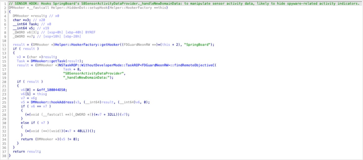


")