Just a few months in the past, whereas engaged on the Databricks with R workshop, I got here
throughout a few of their customized SQL features. These explicit features are
prefixed with “ai_”, and so they run NLP with a easy SQL name:
This was a revelation to me. It showcased a brand new approach to make use of
LLMs in our each day work as analysts. To-date, I had primarily employed LLMs
for code completion and growth duties. Nonetheless, this new strategy
focuses on utilizing LLMs immediately towards our information as an alternative.
My first response was to attempt to entry the customized features by way of R. With dbplyr we are able to entry SQL features
in R, and it was nice to see them work:
One draw back of this integration is that despite the fact that accessible via R, we
require a dwell connection to Databricks with a view to make the most of an LLM on this
method, thereby limiting the quantity of people that can profit from it.
Based on their documentation, Databricks is leveraging the Llama 3.1 70B
mannequin. Whereas it is a extremely efficient Massive Language Mannequin, its monumental measurement
poses a major problem for many customers’ machines, making it impractical
to run on normal {hardware}.
Reaching viability
LLM growth has been accelerating at a fast tempo. Initially, solely on-line
Massive Language Fashions (LLMs) have been viable for each day use. This sparked issues amongst
firms hesitant to share their information externally. Furthermore, the price of utilizing
LLMs on-line may be substantial, per-token fees can add up rapidly.
The best answer can be to combine an LLM into our personal methods, requiring
three important elements:
A mannequin that may match comfortably in reminiscence
A mannequin that achieves adequate accuracy for NLP duties
An intuitive interface between the mannequin and the consumer’s laptop computer
Up to now 12 months, having all three of those parts was almost inconceivable.
Fashions able to becoming in-memory have been both inaccurate or excessively gradual.
Nonetheless, current developments, comparable to Llama from Meta
and cross-platform interplay engines like Ollama, have
made it possible to deploy these fashions, providing a promising answer for
firms trying to combine LLMs into their workflows.
The challenge
This challenge began as an exploration, pushed by my curiosity in leveraging a
“general-purpose” LLM to supply outcomes akin to these from Databricks AI
features. The first problem was figuring out how a lot setup and preparation
can be required for such a mannequin to ship dependable and constant outcomes.
With out entry to a design doc or open-source code, I relied solely on the
LLM’s output as a testing floor. This introduced a number of obstacles, together with
the quite a few choices obtainable for fine-tuning the mannequin. Even inside immediate
engineering, the probabilities are huge. To make sure the mannequin was not too
specialised or centered on a selected topic or end result, I wanted to strike a
delicate stability between accuracy and generality.
Luckily, after conducting intensive testing, I found {that a} easy
“one-shot” immediate yielded the perfect outcomes. By “greatest,” I imply that the solutions
have been each correct for a given row and constant throughout a number of rows.
Consistency was essential, because it meant offering solutions that have been one of many
specified choices (constructive, damaging, or impartial), with none further
explanations.
The next is an instance of a immediate that labored reliably towards
Llama 3.2:
>>> You're a useful sentiment engine. Return solely one of many
... following solutions: constructive, damaging, impartial. No capitalization.
... No explanations. The reply relies on the next textual content:
... I'm blissful
constructive
As a facet notice, my makes an attempt to submit a number of rows directly proved unsuccessful.
The truth is, I spent a major period of time exploring completely different approaches,
comparable to submitting 10 or 2 rows concurrently, formatting them in JSON or
CSV codecs. The outcomes have been typically inconsistent, and it didn’t appear to speed up
the method sufficient to be well worth the effort.
As soon as I turned snug with the strategy, the following step was wrapping the
performance inside an R bundle.
The strategy
Certainly one of my targets was to make the mall bundle as “ergonomic” as potential. In
different phrases, I needed to make sure that utilizing the bundle in R and Python
integrates seamlessly with how information analysts use their most well-liked language on a
each day foundation.
For R, this was comparatively easy. I merely wanted to confirm that the
features labored effectively with pipes (%>% and |>) and could possibly be simply
integrated into packages like these within the tidyverse:
opinions |>llm_sentiment(evaluation) |>filter(.sentiment =="constructive") |>choose(evaluation) #> evaluation#> 1 This has been the perfect TV I've ever used. Nice display, and sound.
Nonetheless, for Python, being a non-native language for me, meant that I needed to adapt my
eager about information manipulation. Particularly, I realized that in Python,
objects (like pandas DataFrames) “include” transformation features by design.
This perception led me to research if the Pandas API permits for extensions,
and luckily, it did! After exploring the probabilities, I made a decision to begin
with Polar, which allowed me to increase its API by creating a brand new namespace.
This straightforward addition enabled customers to simply entry the required features:
>>>import polars as pl>>>import mall>>> df = pl.DataFrame(dict(x = ["I am happy", "I am sad"]))>>> df.llm.sentiment("x")form: (2, 2)┌────────────┬───────────┐│ x ┆ sentiment ││ --- ┆ --- ││ str ┆ str │╞════════════╪═══════════╡│ I'm blissful ┆ constructive ││ I'm unhappy ┆ damaging │└────────────┴───────────┘
By preserving all the brand new features inside the llm namespace, it turns into very simple
for customers to seek out and make the most of those they want:
What’s subsequent
I feel it is going to be simpler to know what’s to come back for mall as soon as the neighborhood
makes use of it and offers suggestions. I anticipate that including extra LLM again ends will
be the principle request. The opposite potential enhancement will probably be when new up to date
fashions can be found, then the prompts could must be up to date for that given
mannequin. I skilled this going from LLama 3.1 to Llama 3.2. There was a necessity
to tweak one of many prompts. The bundle is structured in a approach the longer term
tweaks like that will probably be additions to the bundle, and never replacements to the
prompts, in order to retains backwards compatibility.
That is the primary time I write an article concerning the historical past and construction of a
challenge. This explicit effort was so distinctive due to the R + Python, and the
LLM features of it, that I figured it’s value sharing.
A risk actor referred to as TigerJack is consistently concentrating on builders with malicious extensions printed on Microsoft’s Visible Code (VSCode) market and OpenVSX registry to steal cryptocurrency and plant backdoors.
Two of the extensions, faraway from VSCode after counting 17,000 downloads, are nonetheless current on OpenVSX. Moreover, TigerJack republishes the identical malicious code beneath new names on the VSCode market.
OpenVSX is a community-maintained open-source extension market working as a substitute for Microsoft’s platform, offering an unbiased, vendor-neutral registry.
It is usually the default market for standard VSCode-compatible editors which are technically or legally restricted from VSCode, together with Cursor and Windsurf.
The marketing campaign was noticed by researchers at Koi Safety and has distributed a minimum of 11 malicious VSCode extensions because the starting of the yr.
The 2 of these extensions kicked from the VSCode market are named C++ Playground and HTTP Format, and have been reintroduced on the platform by way of new accounts, the researchers say.
When launched, C++ Playground registers a listener (‘onDidChangeTextDocument’) for C++ recordsdata to exfiltrate supply code to a number of exterior endpoints. The listener fires about 500 milliseconds after edits to seize keystrokes in near-real time.
In accordance with Koi Safety, HTTP Format works as marketed however secretly runs a CoinIMP miner within the background, utilizing hardcoded credentials and configuration to mine crypto utilizing the host’s processing energy.
The miner doesn’t seem to implement any restrictions for useful resource utilization, leveraging your entire computing energy for its exercise.
Miner lively on the host Supply: Koi Safety
One other class of malicious extensions from TigerJack (cppplayground, httpformat, and pythonformat) fetch JavaScript code from a hardcoded deal with and executes it on the host.
The distant deal with (ab498.pythonanywhere.com/static/in4.js) is polled each 20 minutes, enabling arbitrary code execution with out updating the extension.
Malicious operate Supply: Koi Safety
The researchers remark that, not like the supply code stealer and crypto miner, this third kind is way extra menacing, as they function prolonged performance.
“TigerJack can dynamically push any malicious payload with out updating the extension—stealing credentials and API keys, deploying ransomware, utilizing compromised developer machines as entry factors into company networks, injecting backdoors into your initiatives, or monitoring your exercise in real-time.” – Koi Safety
Malicious extension faraway from VSCode (left) however nonetheless obtainable on OpenVSX (proper) Supply: Koi Safety
The researchers say that TigerJack is “a coordinated multi-account operation” disguised by the phantasm of unbiased builders with credible background similar to GitHub repositories, branding, detailed function lists, and extension names that resemble these of authentic instruments.
Koi Safety reported their findings to OpenVSX, however the registry maintainer has not responded by publication time and the 2 extensions stay obtainable for obtain.
Builders utilizing the platform to supply software program are suggested to solely obtain packages from respected and reliable publishers.
Be a part of the Breach and Assault Simulation Summit and expertise the way forward for safety validation. Hear from high specialists and see how AI-powered BAS is reworking breach and assault simulation.
Do not miss the occasion that can form the way forward for your safety technique
This submit discusses my workflow for finishing a revise and resubmit.
I’ve a template doc for representing revise and resubmit responses.
See my templates web page on
github and particularly see
the file “response-to-reviewers.dotx”.
Organising the Response Doc
The doc has the next core types:
Heading 1: Divides up main sections of the evaluation (e.g., Editor, Reviewer 1,
Reviewer 2
Heading 2: Abstract assertion for every reviewer actions
Reviewer Remark: Precise quote of a selected reviewer remark
Physique textual content: For recording my response
Quote: For formatting quotes of particularly modified sections of the textual content
Step 1 is to stick the complete textual content of the editor and reviewers into a brand new Phrase
response doc. Apply reviewer remark fashion
Step 2 is to arrange the response doc. Stage 1 headings are added that
divide up the the reviewer sections.
Reviewer feedback are divided into discrete factors.
The division of revision factors might or will not be clear.
Some reviewers present numbered factors. Others present a extra narrative evaluation
the place every paragraph consists of a number of factors. Some factors are interconnected
however contain distinct actions. For every level that’s recognized, I add a stage 2 heading. The extent 2 heading
consists of an identifier and a quick abstract assertion of the requirement.
Identifiers are for instance, “R1.2”, which might check with reviewer 1’s second
level. In some circumstances, the place there are related factors, you get “R1.2.1”,
“R1.2.2” and so forth.
There are a number of advantages to utilizing identifiers. In some circumstances, a number of
reviewers make the identical level. Thus, you’ll be able to rapidly refer the reviewer to
one other evaluation level. E.g., “This level was addressed in reviewer level R1.2”.
It will also be an environment friendly manner of protecting observe of reviewer factors if you end up
working by a lot of them.
The abstract statements are vital. I goal to maintain them brief. Ideally they will
match on one line in order that they’re simple to rapidly perceive (i.e., round 50
characters). I attempt to make them instructions. For instance:
Make clear distinctive contribution
Enhance research motivation in introduction
Describe x extra clearly
Add references to …
Justify statistical methodology
Think about using … methodology
Embody … Desk 1
In some circumstances, the required motion shouldn’t be explicitly acknowledged by the reviewer. For
instance, if a reviewer critiques a methodological choice, there are numerous
doable actions together with, justifying your alternative, including a limitation, and so
on.
Advantages of the above strategy
Utilizing formal Headings in MS Phrase lets you view a doc
map on the aspect that may rapidly will let you navigate between reviewer factors.
One other good thing about the above course of is that reviewer feedback begin to seem
extra manageable. Once you first obtain a number of pages of reviewer feedback, it may well
really feel overwhelming. The above course of begins to divide up every level right into a extra
manageable activity. The act of offering a abstract assertion additionally forces you to
learn and perceive what motion is required to answer the reviewer remark.
Report preliminary reflections
Above, I present how the primary studying is used to parse reviewer feedback into discrete factors and provides descriptive titles. Within the second studying, I add feedback to every reviewer level utilizing the remark function within the Phrase Processor. This is a chance to have some preliminary reflections on (a) how simple will probably be to fulfill the revision, (b) whether or not a change to the manuscript is required, and (c) what needs to be completed. After I’ve added these, I typically flow into the response doc to collaborators, to permit them so as to add feedback.
Sequencing the Revisions
The following activity is to find out a sequence for working by the revisions.
This includes protecting observe of which factors nonetheless should be addressed and
deciding on an order to work by the factors.
At a primary stage, I place an asterisk initially of every heading that has not
but been addressed. That is eliminated as soon as the purpose has been adequately
addressed.
A more difficult challenge is deciding on the way to work by the
modifications. Some modifications are interdependent. Nonetheless, main revisions typically
should be labored by first as they will have broader structural implications
for the manuscript. A couple of helpful steps for desirous about sequencing embrace:
Organise the factors into classes
Learn by every level, and make some tentative notes about what to do (e.g., utilizing feedback in Phrase).
Resolve on an specific sequence to work on the factors. This typically requires you
to brainstorm the professionals and cons of engaged on one level versus one other first.
In some circumstances, sequencing will elevate some extra meta-issues concerning the paper that
transcend any given evaluation level. I principally discover it best to work by factors within the following order: analyses, outcomes, methodology, introduction, dialogue. The rationale is that any new analyses that you simply run and incorporate into your paper will change your outcomes. And these might additional require modifications to the tactic, which in flip affect the framing and dialogue. Likewise, if the introduction is modified, this will have implications for a way the dialogue integrates subjects raised within the introduction.
Logistically, I generate a desk of contents in MS Phrase. This lists all of the reviewer level titles (i.e., the IDs and the titles similar to “R1.1 Replace methodology to incorporate …”). This works as a result of all of the reviewer factors are formatted utilizing heading types. I then copy and paste this as plain textual content into a piece doc. These factors are then organised thematically below headings and into an acceptable sequential order.
Addressing Revision Factors
If sequencing points have been resolved, it’s a matter of working by every
revision level. I’ve a number of guiding rules:
Write in a way which focuses on the scientific challenge.
Deal with the reviewer with respect.
If a reviewer has misunderstood one thing within the manuscript, take duty
for making the manuscript clearer.
One other level is that the response doc needs to be self-contained. Ideally,
the reviewer shouldn’t want to take a look at the precise manuscript to guage whether or not
you’ve got successfully responded to their requested modifications. This makes the expertise of the
reviewer rather more nice. From a strategic perspective, they could even be much less
inclined to learn by the whole manuscript once more and give you all new
considerations.
If a desk or determine is up to date, then paste a screenshot of the up to date desk
or determine.
If a brand new paragraph has been added, embrace a replica of that paragraph.
If a sentence or two has been added to a paragraph, embrace a replica of the
complete paragraph and daring the part that has been added.
Provided that the purpose could be very primary is it ample to say, “this variation was
made”. Examples of this is perhaps including a reference, fixing up typos, and so
on.
One other helpful technique is to point new textual content within the manuscript with a unique color font (e.g., purple).
Collaborations and Revisions
It’s typically best if one individual leads revisions.
The lead individual can even allocate particular revision duties to co-authors. There may be the problem of the way to synchronise the revisions within the manuscript with the response doc. If the modifications are significantly complicated or the collaborators are more likely to make substantial extra modifications to the manuscript, then it could be value ready a bit of bit earlier than finishing the response doc. Or alternatively simply see the response doc as an preliminary draft to be returned as soon as the manuscript has been finalised.
Monitor Modifications
Some journals require that you simply embrace a model of the manuscript with observe modifications. In different circumstances, it may well simply be a helpful addition to the submission. In case you are utilizing MS Phrase, then the evaluate paperwork function is good for producing this doc. This function lets you anonymise the change as a result of you’ll be able to label the change with “creator” quite than your precise title.
Narrator: Have you ever ever thought of how your physique turns meals into power or simply how rigorously it has to handle that course of?
After we eat, the glucose from our meals will get saved within the liver as glycogen.
On supporting science journalism
For those who’re having fun with this text, think about supporting our award-winning journalism by subscribing. By buying a subscription you might be serving to to make sure the way forward for impactful tales concerning the discoveries and concepts shaping our world as we speak.
And primarily based on our physique’s wants, the liver will convert that glycogen again into glucose, in order that it might journey via the blood and get to our cells, which flip that glucose into power.
In the meantime our pancreas produces a hormone referred to as insulin, whose job is to enter the blood and inform our cells to absorb that glucose.
That additionally makes insulin a regulator of our physique’s blood sugar ranges, stopping the issues that may occur when our ranges are too excessive or too low.
When the pancreas stops producing insulin, glucose doesn’t enter our cells. As an alternative it accumulates within the bloodstream.
In some individuals, the pancreas stops making insulin altogether.
This situation is named Kind 1 Diabetes.
Kind 1 Diabetes is usually referred to as juvenile diabetes as a result of it usually makes its look in childhood or adolescence.
Whereas the precise trigger is mysterious, we all know the illness occurs as a result of immune cells goal and assault insulin-producing cells within the pancreas referred to as beta cells.
As these cells get destroyed, the physique stops producing insulin and loses that key regulator of blood sugar ranges.
That in flip can drive plenty of signs, together with fatigue and weak spot.
Rising blood glucose ranges trigger the physique to search for different methods to eliminate extra sugar, like frequent urination.
That in flip requires the physique to attract water from different locations, such because the pores and skin and eyes, resulting in dry mouth and pores and skin and likewise imaginative and prescient modifications.
Folks may additionally really feel very thirsty as their physique alerts the necessity for extra water.
Excessive blood sugar ranges may also trigger poor blood circulate, making it troublesome for the physique to heal sores and different wounds.
And a few individuals may additionally expertise a sort of nerve injury generally known as diabetic neuropathy, which might result in numbness or ache in areas such because the chest or fingers.
Our understanding of diabetes goes again millennia.
Historical data from India and China documented some sort of situation with a really curious symptom: pee that tasted candy.
Numerous texts included different signs as nicely, comparable to extreme thirst and speedy weight reduction.
One of many earliest references to the time period “diabetes” dates to the second century C.E., when the Greek doctor Aretaeus famous the time period and mentioned it drew from the Greek phrase diabaino.
It means “I cross via,” in reference to the extreme urine.
In his writing, he famous that whereas it may take a very long time for the situation to type, individuals died rapidly as soon as it had established itself.
As remedy, he steered consuming cereals, milk and wine.
Regardless of these early observations of diabetes, it might take a very long time for docs and scientists to know the situation nicely sufficient to make it much less deadly.
Within the seventeenth century the English doctor Thomas Willis expanded the title to “diabetes mellitus.”
The addition of “mellitus” drew on the Latin phrase mel, for honey, to as soon as once more emphasize the candy style of urine that was related to diabetes.
And in 1776 a doctor named Matthew Dobson traced that sweetness to the presence of sugar within the urine.
Over the subsequent few centuries, scientists would uncover the organs and molecules that led to that extra sugar.
Within the nineteenth century Claude Bernard uncovered the significance of the liver in regulating blood sugar ranges.
A number of a long time later Joseph von Mering and Oskar Minkowski found that eradicating the pancreas from a canine led to the event of diabetes.
Shortly after that, Edward Albert Sharpey-Schafer hypothesized that diabetes was the results of a deficiency in a single chemical made in a area of the pancreas referred to as the islets of Langerhans.
He referred to as this chemical insulin, counting on the Latin phrase “insula” for island to present credit score to these islet cells.
However the precise discovery of insulin was the work of Frederick Banting and Charles Finest, who, in 1921, discovered that they might reverse diabetes in canines by introducing pancreatic cells from wholesome canines.
They might later work with James Collip and John Macleod to purify insulin from cow pancreases, and in 1922 a 14 12 months outdated boy named Leonard Thompson acquired one of many first insulin injections to deal with diabetes.
He would go on to dwell 13 years earlier than dying of pneumonia.
Over the twentieth and twenty first centuries, scientists have developed applied sciences which have made kind 1 diabetes treatable.
These embody meters to examine blood glucose ranges and pumps that give small doses of insulin.
And with advances in development and software program, these instruments have develop into smaller and extra moveable.
Regardless of these advances, scientists are nonetheless pursuing a remedy for kind 1 diabetes.
The historical past of kind 1 diabetes reveals how we have now managed to take a illness that was as soon as deadly and make it treatable.
And as scientists make extra advances, their work displays the hope and risk that sooner or later, this illness will develop into curable.
C. J. Van Hook, “Hantavirus pulmonary syndrome—the twenty fifth anniversary of the 4 Corners outbreak,” Emerg. Infect. Dis., vol. 24, no. 11, pp. 2056–2060, 2018.
[2]
CDC, “About zoonotic ailments,” One Well being, 01-July-2025. [Online]. Accessible: https://www.cdc.gov/one-health/about/about-zoonotic-diseases.html. [Accessed: 24-Aug-2025].
C. J. Carlson et al., “Local weather change will increase cross-species viral transmission danger,” Nature, vol. 607, no. 7919, pp. 555–562, 2022.
[5]
A. Borham et al., “Local weather change and zoonotic illness outbreaks: Rising proof from epidemiology and toxicology,” Int. J. Environ. Res. Public Well being, vol. 22, no. 6, 2025.
[6]
R. A. Weiss and N. Sankaran, “Emergence of epidemic ailments: zoonoses and different origins,” Fac. Rev., vol. 11, p. 2, 2022.
[7]
M. N. Hayek, “The infectious illness entice of animal agriculture,” Sci. Adv., vol. 8, no. 44, p. eadd6681, 2022.
[8]
R. Okay. Plowright et al., “Pathways to zoonotic spillover,” Nat. Rev. Microbiol., vol. 15, no. 8, pp. 502–510, 2017.
[9]
J. E. B. Halliday et al., “Zoonotic causes of febrile sickness in malaria endemic international locations: a scientific evaluate,” Lancet Infect. Dis., vol. 20, no. 2, pp. e27–e37, 2020.
[10]
L. H. Taylor, S. M. Latham, and M. E. Woolhouse, “Threat elements for human illness emergence,” Philos. Trans. R. Soc. Lond. B Biol. Sci., vol. 356, no. 1411, pp. 983–989, 2001.
[11]
S. Pauciullo, V. Zulian, S. La Frazia, P. Paci, and A. R. Garbuglia, “Spillover: Mechanisms, genetic limitations, and the position of reservoirs in rising pathogens,” Microorganisms, vol. 12, no. 11, 2024.
[12]
W. Ma, R. E. Kahn, and J. A. Richt, “The pig as a mixing vessel for influenza viruses: Human and veterinary implications,” J. Mol. Genet. Med., vol. 3, no. 1, pp. 158–166, 2008.
[13]
F. S. Flores, C. Zanluca, A. A. Guglielmone, C. N. Duarte Dos Santos, M. B. Labruna, and A. Diaz, “Vector competence for West Nile virus and St. Louis encephalitis virus (Flavivirus) of three tick species of the genus Amblyomma (Acari: Ixodidae),” Am. J. Trop. Med. Hyg., vol. 100, no. 5, pp. 1230–1235, 2019.
[14]
X. Guo et al., “Molecular markers and mechanisms of influenza A virus cross-species transmission and new host adaptation,” Viruses, vol. 16, no. 6, p. 883, 2024.
[15]
J. Wang et al., “A scientific evaluate and meta-analysis of the sources of Salmonella in poultry manufacturing (pre-harvest) and their relative contributions to the microbial danger of poultry meat,” Poult. Sci., vol. 102, no. 5, p. 102566, 2023.
[16]
CDC, “Cryptosporidiosis NNDSS Abstract Report for 2022,” Waterborne Illness and Outbreak Surveillance Reporting, 21-Aug-2025. [Online]. Accessible: https://www.cdc.gov/healthy-water-data/documentation/cryptosporidiosis-nndss-summary-report-for-2022.html. [Accessed: 26-Aug-2025].
“Mpox 2022 to 2025 Replace: A Complete Evaluation on Its Issues, Transmission, Prognosis, and Therapy,” Mdpi.com. [Online]. Accessible: https://www.mdpi.com/1999-4915/17/6/753. [Accessed: 26-Aug-2025].
[19]
“Investigation of Heartland Virus Illness All through the US, 2013–2017,” Oup.com. [Online]. Accessible: https://tutorial.oup.com/ofid/article/7/5/ofaa125/5819209. [Accessed: 26-Aug-2025].
[20]
D. L. Zychowski, G. Bamunuarachchi, S. P. Commins, R. M. Boyce, and A. C. M. Boon, “Proof of human Bourbon virus infections, North Carolina, USA,” Emerg. Infect. Dis., vol. 30, no. 11, pp. 2396–2399, 2024.
[21]
C. J. Carlson, C. M. Zipfel, R. Garnier, and S. Bansal, “World estimates of mammalian viral range accounting for host sharing,” Nat. Ecol. Evol., vol. 3, no. 7, pp. 1070–1075, 2019.
This weblog introduces retrospective simulation, impressed by Taleb’s “FooledbyRandomness,” to simulate 1,000 alternate historic worth paths utilizing a non-parametric Brownian bridge methodology. Utilizing SENSEX knowledge (2000–2020) as in-sample knowledge, the writer optimises an EMA crossover technique throughout the in-sample knowledge first, after which applies it to the out-of-sample knowledge utilizing the optimum parameters obtained from the in-sample backtest. Whereas the technique outperforms the buy-and-hold strategy in in-sample testing, it considerably underperforms in out-of-sample testing (2020–2025), highlighting the chance of overfitting to a single realised path. The writer then runs the backtest throughout all simulated paths to establish essentially the most regularly profitable SEMA-LEMA parameter mixtures.
The writer additionally calculates VaR and CVaR utilizing over 5 million simulated returns and compares return extremes and distributional traits, revealing heavy tails and excessive kurtosis. This framework permits extra strong technique validation by evaluating how methods would possibly carry out throughout a number of believable market eventualities.
Introduction
In “Fooled by Randomness”, Taleb says at one place, “To start with, after I knew near nothing (that’s, even lower than at this time), I questioned whether or not the time sequence reflecting the exercise of individuals now lifeless or retired ought to matter for predicting the long run.”
This bought me pondering. We frequently run simulations for the possible paths a time sequence can take sooner or later. Nonetheless, the premise for these simulations relies on historic knowledge. Given the stochastic nature of asset costs (learn extra), the realised worth path had the selection of an infinite variety of paths it might have taken, however it traversed by way of solely a kind of infinite potentialities. And I assumed to myself, why not simulate these alternate paths?
In frequent follow, this strategy is known as bootstrap historic simulation. I selected to discuss with it as retrospective simulation, as a extra intuitive counterpart to the phrases ‘look-ahead’ and ‘walk-forward’ used within the context of simulating the long run.
Article map
Right here’s an overview of how this text is laid out:
Knowledge Obtain
We import the required libraries and obtain the every day knowledge of the SENSEX index, a broad market index based mostly on the Bombay Inventory Trade of India.
I’ve downloaded the info from January 2000 to November 2020 because the in-sample knowledge, and from December 2020 to April 2025 because the out-of-sample knowledge. We might have put in a spot (an embargo) between the in-sample and out-of-sample knowledge to minimise, if not eradicate, knowledge leakage (learn extra). In our case, there’s no direct knowledge leakage. Nonetheless, since inventory ranges (costs) are identified to bear autocorrelation, like we noticed above, the SENSEX index on the primary buying and selling day of December 2020 could be extremely correlated with its degree on the final buying and selling day of November 2020.
Thus, once we practice our mannequin on knowledge that features the final buying and selling day of November 2020, it extracts info from that day’s degree and makes use of it to get educated. Since our testing dataset is from the primary buying and selling day of December 2020, some residual info from the coaching dataset is current within the testing dataset.
As an extension, the coaching set accommodates some info that can also be current within the testing dataset. Nonetheless, this info will diminish over time and finally change into insignificant. Having mentioned that, I didn’t keep a spot between the in-sample and out-of-sample datasets in order that we are able to give attention to understanding the core idea of this text.
You should utilize any yfinance ticker to obtain knowledge for an asset of your liking. You can even modify the dates to fit your wants.
The subsequent half is the primary crux of this weblog. That is the place I simulate the potential paths the asset might have taken from January 2000 to November 2020. I’ve simulated 1000 paths. You possibly can modify it to make it 100 or 10000, as you want. The upper the worth, the better our confidence within the outcomes, however there’s a tradeoff in computational time. I’ve simulated solely the closing costs. I saved the first-day and last-day costs the identical because the realised ones, and simulated the in-between costs.
Retaining the worth mounted on the primary day is sensible. However the final day? If the costs are to observe a random stroll (learn extra), the closing worth ranges of most, if not all, paths needs to be completely different, isn’t it? However I made an assumption right here. Given the environment friendly market speculation, the index would have a good worth by the tip of November 2020, and after shifting on its capricious course, it might converge again to this honest worth.
Why solely November 2020?
Was the extent of the index at its fairest worth at the moment? No means of understanding. Nonetheless, one date is nearly as good as another, and we have to work with a particular date, so I selected this one.
One other consideration right here is on what foundation we permit the simulated paths to meander. Ought to or not it’s parametric, the place we assume the time sequence to observe a particular distribution, or non-parametric, the place we don’t make any such assumption? I selected the latter. The monetary literature discusses costs (and their returns) as belonging roughly to sure underlying distributions. Nonetheless, in the case of outlier occasions, akin to extremely risky worth jumps, these assumptions start to interrupt down, and it’s these occasions {that a} quant (dealer, portfolio supervisor, investor, analyst, or researcher) needs to be ready for.
For the non-parametric strategy, I’ve modified the Brownian bridge strategy. In a pure Brownian bridge strategy, the returns are assumed to observe a Gaussian distribution, which once more turns into considerably parametric (learn extra). Nonetheless, in our strategy, we calculate the realized returns from the in-sample closing costs and use these returns as a pattern for the simulation generator to select from. We’re utilizing bootstrapping with alternative (learn extra), which signifies that the realized returns aren’t simply being shuffled; some values could also be repeated, whereas some might not be used in any respect. If the values are merely shuffled, all simulated paths would land on the final closing worth of the in-sample knowledge. How will we make sure that the simulated costs converge to the ultimate shut worth of the in-sample knowledge? We’ll use geometric smoothing for that.
One other consideration: since we use the realized returns, we’re priming the simulated paths to resemble the realized path, appropriate? Form of, but when we had been to generate pseudo-random numbers for these returns, we must make some assumption about their distribution, making the simulation a parametric course of.
Right here’s the code for the simulations:
Be aware that I didn’t use a random seed when producing the simulated paths. I’ll point out the rationale at a later stage.
Let’s plot the simulated paths:
The above graph exhibits that the beginning and ending costs are the identical for all 1,000 simulated paths. We must always word one factor right here. Since we’re working with knowledge from a broad market index, whose ranges depend upon many interlinked macroeconomic variables and elements, it is extremely unlikely that the index would have traversed a lot of the paths simulated above, given the identical macroeconomic occasions that occurred through the simulation interval. We’re making an implicit assumption right here that the required macroeconomic variables and elements differ in every of the simulated paths, and the interactions between these variables and elements outcome within the simulated ranges that we generate. This holds for another asset class or asset you resolve to exchange the SENSEX index with, for retrospective simulation functions.
Exponential Transferring Common Crossover Technique Improvement and Backtesting on In-Pattern Knowledge, and Parameter Optimisation
Subsequent, we develop a easy buying and selling technique and conduct a backtest utilizing the in-sample knowledge. The technique is a straightforward exponential shifting common crossover technique, the place we go lengthy when the short-period exponential shifting common (SEMA) of the shut worth goes above the long-period exponential shifting common (LEMA), and we go quick when the SEMA crosses the LEMA from above (learn extra).
By optimisation, we’ll try to seek out the very best SEMA and LEMA mixture that yields the utmost returns. For the SEMA, I take advantage of lookback durations of 5, 10, 15, 20, … as much as 100, and for the LEMA, 20, 30, 40, 50, … as much as 300.
The situation is that for any given SEMA and LEMA mixture, the LEMA lookback interval needs to be better than the corresponding SEMA lookback interval. We might carry out backtests on all completely different mixtures of those SEMA and LEMA values and select the one which yields the very best efficiency.
We’ll plot:
the fairness curve of the technique with the best-performing SEMA and LEMA lookback values, plotted towards the buy-and-hold fairness,
the purchase and promote alerts plotted together with the shut costs of the in-sample knowledge and the SEMA and LEMA strains,
the underwater plot of the technique, and,
a heatmap of the returns for various LEMA and SEMA calculations.
We’ll calculate:
the SEMA and LEMA lookback values for the best-performing mixture,
the whole returns of the technique,
the utmost drawdown of the technique, and,
the Sharpe ratio of the technique.
We may also overview the highest 10 SEMA and LEMA mixtures and their respective performances.
Right here’s the code for all the above:
And listed below are the outputs of the above code:
Greatest SEMA: 5, Greatest LEMA: 40
Whole Return: 873.43%
Most Drawdown: -41.28 %
Sharpe Ratio: 0.59
The heatmap exhibits a gradual change in colour from one adjoining cell to the subsequent. This implies that slight modifications to the EMA values don’t result in drastic adjustments within the technique’s efficiency. After all, it might be extra gradual if we had been to scale back the spacing between the SEMA values from 5 to, say, 2, and between the LEMA values from 10 to, say, 3.
The technique outperforms the buy-and-hold technique, as proven within the fairness plot. Excellent news, proper? Be aware right here that this was in-sample backtesting. We ran the optimisation on a given dataset, took some info from it, and utilized it to the identical dataset. It’s like utilizing the costs for the subsequent 12 months (that are unknown to us now, besides for those who’re time-travelling!) to foretell the costs over the subsequent 12 months. Nonetheless, we are able to utilise the knowledge gathered from this dataset to use it to a different dataset. That’s the place we use the out-of-sample knowledge.
Backtesting on Out-of-Pattern Knowledge
Let’s run the backtest on the out-of-sample dataset:
Earlier than we see the outputs of the above codes, let’s listing what we’re doing right here.
We’re plotting:
The fairness curve of the technique plotted alongside that of the buy-and-hold, and,
The underwater plot of the technique.
We’re calculating:
Technique returns,
Purchase-and-hold returns,
Technique most drawdown,
Technique Sharpe ratio,
Purchase-and-hold Sharpe ratio, and,
Technique hit ratio.
For the Sharpe ratio calculations, we assume a risk-free price of return of 0. Listed below are the outputs:
The technique underperforms the underlying by a major margin. However that’s not what we’re primarily interested by, so far as this weblog is worried. We have to think about that we ran an optimisation on solely one of many many paths that the costs might have taken through the in-sample interval, after which extrapolated that to the out-of-sample backtest. That is the place we use the simulation we carried out in the beginning. Let’s run the backtest on the completely different simulated paths and test the outcomes.
Backtesting on Simulated Paths and Optimising to Extract the Greatest Parameters
This may hold printing the corresponding SEMA and LEMA values for the very best technique efficiency, and the efficiency itself for the simulated paths:
Accomplished optimization for column 0: SEMA=65, LEMA=230, Return=1.8905
Accomplished optimization for column 1: SEMA=45, LEMA=140, Return=4.4721
.....................................................................
Accomplished optimization for column 998: SEMA=10, LEMA=20, Return=3.6721
Accomplished optimization for column 999: SEMA=15, LEMA=20, Return=9.8472
Right here’s a snap of the output of this code:
Now, we’ll kind the above desk in order that the SEMA and LEMA mixture with the very best returns for essentially the most paths is on the prime, adopted by the second-best mixture, and so forth.
Let’s test how the desk would look:
Right here’s a snapshot of the output:
Of the 1000 paths, 47 confirmed the very best returns with a mix of SEMA 5 and LEMA 20. Since I didn’t use a random seed whereas producing the simulated paths, you possibly can run the code a number of instances and procure completely different outputs or outcomes. You’ll see that the very best SEMA and LEMA mixture within the above desk would more than likely be 5 and 20. The frequencies can change, although.
How do I do know?
As a result of I’ve performed so, and have gotten the mixture of 5 and 20 within the first place each time (adopted by 100 and 300 within the second place). After all, it’s not that there’s a zero probability of getting another mixture within the prime row.
Out-of-Pattern Backtesting utilizing Optimised Parameters based mostly on Simulated Knowledge Backtesting
We’ll extract the SEMA and LEMA look-back mixture from the earlier step that yields the very best returns for a lot of the simulated paths. We’ll use a dynamic strategy to automate this choice. Thus, if as an alternative of 5 and 20, we had been to acquire, say, 90 and 250 because the optimum mixture, the identical could be chosen, and the backtest could be carried out utilizing that.
Let’s use this mixture to run an out-of-sample backtest:
Right here, the technique not solely underperforms the underlying but in addition generates adverse returns. So what’s the purpose of all this effort that we put in? Let’s word that I employed the shifting common crossover technique to illustrate the applying of retrospective simulation utilizing a modified Brownian bridge. This strategy is extra appropriate for testing complicated methods with a number of circumstances, and machine studying (ML)-based and deep studying (DL)-based methods.
We’ve got approaches akin to walk-forward optimisation and cross-validation to beat the issue of optimising or fine-tuning a technique or mannequin on solely one of many many potential traversable paths.
Nonetheless, this strategy of retrospective simulation ensures that you simply don’t must depend on just one path however can make use of a number of retrospective paths. Nonetheless, since operating an ML-based technique on these simulated paths could be too computationally intensive for many of our readers who don’t have entry to GPUs or TPUs, I selected to work with a easy technique.
Moreover, for those who want to modify the strategy, I’ve included some options on the finish.
Analysis of VaR and C-VaR
Let’s transfer on to the subsequent half. We’ll utilise the retrospective simulation to calculate the worth in danger and the conditional worth in danger (learn extra: 1, 2, 3).
Let’s decipher the above output. We first calculated the every day % returns of all 1000 simulated paths. Each path has 5,155 days of knowledge, which yielded 5,154 returns per path. When multiplied by 1,000 paths, this resulted in 5,154,000 values of every day returns. We used all these values and located the bottom ninetieth, ninety fifth, and 99th percentile values, respectively.
From the above output, for instance, we are able to say with 95% certainty that if the long run costs observe paths just like these simulated paths, the utmost drawdown that we are able to face on any given day could be 2.21%. The anticipated drawdown could be 3.53% if that degree will get breached.
Let’s speak concerning the extremes now. Let’s evaluate the utmost and minimal every day returns of the simulated paths and the realised in-sample path.
Realized Lowest Day by day Return: -0.1315258002691394
Realized Highest Day by day Return: 0.17339334818061447
The utmost values from each approaches are shut, at round 17.4%. Similar for the minimal values, at round -13.2%. This makes a case for utilizing this strategy in monetary modelling.
Distribution of Simulated Knowledge
Let’s see how the simulated returns are distributed and evaluate them visually to a standard distribution. We’ll additionally calculate the skewness and the kurtosis.
The argument ‘kde’, when set to ‘True’, smooths the histogram curve, as proven within the above plot. Additionally, in order for you a extra granular (coarse) visible of the distribution, you possibly can enhance (scale back) the worth within the ‘bins’ argument.
Although the histogram resembles a bell curve, it’s removed from a standard distribution. It reveals heavy kurtosis, that means there are important probabilities of discovering returns which might be many normal deviations away from the imply. And this isn’t any shock, since that’s how fairness and equity-index returns are inherently.
The place This Method Can Be Most Helpful
Whereas the technique I used right here is straightforward and illustrative, this retrospective simulation framework comes into its personal when utilized to extra complicated or nuanced methods. It’s helpful in circumstances the place:
You are testing multi-condition or ML-based fashions which may overfit on a single realized path.
You need to stress take a look at a technique throughout alternate historic realities—ones that didn’t occur, however very properly might have.
Conventional walk-forward or cross-validation strategies don’t appear to be sufficient, and also you need an added lens to consider generalisability.
You are exploring how a technique would possibly behave (or may need behaved had the worth taken on any alternate worth path) below excessive market strikes that aren’t current within the precise historic path.
In essence, this methodology lets you transition from “what occurred” to “what might have occurred,” a refined but highly effective shift in perspective.
Steered Subsequent Steps
In case you discovered this strategy attention-grabbing, listed below are a number of methods you possibly can prolong it:
Strive extra refined methods: Apply this retrospective simulation to mean-reversion, volatility breakout, or reinforcement learning-based methods.
Introduce macro constraints: Anchor the simulations round identified macroeconomic markers or regime adjustments to check how methods behave in such environments.
Use intermediate anchor factors: As an alternative of simply fixing the beginning and finish costs, attempt anchoring the simulation at quarterly or annual ranges to higher management drift and convergence.
Prepare ML fashions on simulated paths: In case you’re working with supervised studying or deep studying fashions, practice them on a number of simulated realities as an alternative of 1.
Portfolio-level testing: Use this framework to judge VaR, CVaR, or stress-test a whole portfolio, not only a single technique.
That is only the start—the way you construct on it will depend on your curiosity, computing sources, and the questions you are making an attempt to reply.
In Abstract
The weblog launched a retrospective simulation framework utilizing a non-parametric Brownian bridge strategy to simulate alternate historic worth paths.
We employed a easy EMA crossover technique to illustrate how this simulation will be built-in into a standard backtesting loop.
We extracted the finest SEMA and LEMA mixtures after operating backtests on the simulated in-sample paths, after which used these for backtesting on the out-of-sample knowledge.
This simulation methodology permits us to check how methods would behave not solely in response to what occurred, but in addition in response to what might have occurred, serving to us keep away from overfitting and uncover strong alerts.
The identical simulated paths can be utilized to derive distributional insights, akin to tail threat (VaR, CVaR) or return extremes, providing a deeper understanding of the technique’s threat profile.
Often Requested Questions
1. Curious why we simulate worth paths in any respect? Actual market knowledge exhibits solely one path the market took, amongst many potential paths. However what if we need to perceive how our technique would behave throughout many believable realities sooner or later, or would have behaved throughout such realities previously? That’s why we use simulations.
2. What precisely is a Brownian bridge, and why was it used? A Brownian bridge simulates worth actions that begin and finish at particular values, like actual historic costs. This helps guarantee simulated paths are anchored in actuality whereas nonetheless permitting randomness in between. The primary query we ask right here is “What else might have occurred previously?”.
3. What number of simulated paths ought to I generate to make this evaluation significant? We used 1000 paths. As talked about within the weblog, when the variety of simulated paths will increase, computation time will increase, however our confidence within the outcomes grows too.
4. Is that this solely for easy methods like shifting averages? By no means. We used the shifting common crossover simply for example. This framework will be (and needs to be) used if you’re testing complicated, ML-based, or multi-condition methods which will overfit to historic knowledge.
5. How do I discover the very best parameter settings (like SEMA/LEMA)? For every simulated path, we backtested completely different parameter mixtures and recorded the one which gave the best return. By counting which mixtures carried out finest throughout most simulations, we recognized the mixture that’s more than likely to carry out properly. The concept is to not depend on the mixture that works on only one path.
6. How do I do know which parameter combo to make use of within the markets? The concept is to select the combo that the majority regularly yielded the very best outcomes throughout many simulated realities. This helps keep away from overfitting to the only historic path and as an alternative focuses on broader adaptability. The precept right here is to not let our evaluation and backtesting be topic to probability or randomness, however moderately to have some statistical significance.
7. What occurs after I discover that “finest” parameter mixture? We run an out-of-sample backtest utilizing that mixture on knowledge the mannequin hasn’t seen. This checks whether or not the technique works outdoors of the info on which the mannequin is educated.
8. What if the technique fails within the out-of-sample take a look at? That’s okay, and on this instance, it did! The purpose is to not “win” with a fundamental technique, however to indicate how simulation and strong testing reveal weaknesses earlier than actual cash is concerned. After all, if you backtest an precise alpha-generating technique utilizing this strategy and nonetheless get underperformance within the out-of-sample, it doubtless signifies that the technique isn’t strong, and also you’ll must make adjustments to the technique.
9. How can I take advantage of these simulations to grasp potential losses? We adopted the strategy of flattening the returns from all simulated paths into one massive distribution and calculating threat metrics like Worth at Danger (VaR) and Conditional VaR (CVaR). These present how unhealthy issues can get, and the way usually.
10. What’s the distinction between VaR and CVaR?
VaR tells us the worst anticipated loss at a given confidence degree (e.g., “you’ll lose not more than 2.2% on 95% of days”).
CVaR goes a step additional and says, “In case you lose greater than that, right here’s the typical of these worst days.”.
11. What did we study from the VaR/CVaR outcomes on this instance? We noticed that 99% of days resulted in losses no worse than ~4.25%. However when losses exceeded that threshold, they averaged ~5.86%. That’s a helpful perception into tail threat. These are the uncommon however extreme occasions that may extremely have an effect on our buying and selling accounts if not accounted for.
12. Are the simulated return extremes reasonable in comparison with actual markets? Sure, they matched very carefully with the utmost and minimal every day returns from the actual in-sample knowledge. This validates that our simulation isn’t simply random however is grounded in actuality.
13. Do the simulated returns observe a standard distribution? Not fairly. The returns confirmed excessive kurtosis (fats tails) and slight adverse skewness, that means excessive strikes (each up and down) are extra frequent than a standard distribution would have. This mirrors actual market behaviour.
14. Why does this matter for threat administration? If our technique assumes regular returns, we’re closely underestimating the likelihood of great losses. Simulated returns reveal the true nature of market threat, serving to us put together for the surprising.
15. Is that this simply an instructional train, or can I apply this virtually? This strategy is extremely helpful in follow, particularly if you’re working with:
Machine studying fashions which might be susceptible to overfitting
Methods designed for high-risk environments
Portfolios the place stress testing and tail threat are essential
Regime-switching or macro-anchored fashions
It helps shift our mindset from “What labored earlier than?” to “What would have labored throughout many alternate market eventualities?”, and that may be one latent supply of alpha.
Conclusion
Hope you discovered a minimum of one new factor from this weblog. In that case, do share what it’s within the feedback part beneath and tell us for those who’d prefer to learn or study extra about it. The important thing takeaway from the above dialogue is the significance of performing simulations retrospectively and making use of them to monetary modelling. Apply this strategy to extra complicated methods and share your experiences and findings within the feedback part. Blissful studying, glad buying and selling 🙂
Chainika Thakar, thanks for rendering and publishing this, and making it obtainable to the world, that too in your birthday!
Disclaimer: All investments and buying and selling within the inventory market contain threat. Any choice to put trades within the monetary markets, together with buying and selling in inventory or choices or different monetary devices is a private choice that ought to solely be made after thorough analysis, together with a private threat and monetary evaluation and the engagement {of professional} help to the extent you imagine needed. The buying and selling methods or associated info talked about on this article is for informational functions solely.
ML Equipment is a cellular SDK from Google that makes use of machine studying to unravel issues similar to textual content recognition, textual content translation, object detection, face/pose detection, and a lot extra!
The APIs can run on-device, enabling you to course of real-time use instances with out sending information to servers.
ML Equipment supplies two teams of APIs:
Imaginative and prescient APIs: These embrace barcode scanning, face detection, textual content recognition, object detection, and pose detection.
Pure Language APIs: You employ them each time it is advisable establish languages, translate textual content, and carry out good replies in textual content conversations.
This tutorial will give attention to Textual content Recognition. With this API you’ll be able to extract textual content from pictures, paperwork, and digicam enter in actual time.
On this tutorial, you’ll be taught:
What a textual content recognizer is and the way it teams textual content parts.
The ML Equipment Textual content Recognition options.
Learn how to acknowledge and extract textual content from a picture.
Getting Began
All through this tutorial, you’ll work with Xtractor. This app allows you to take an image and extract the X usernames. You might use this app in a convention each time the speaker exhibits their contact information and also you’d prefer to search for them later.
Use the Obtain Supplies button on the high or backside of this tutorial to obtain the starter challenge.
As soon as downloaded, open the starter challenge in Android Studio Meerkat or newer. Construct and run, and also you’ll see the next display:
Clicking the plus button will allow you to select an image out of your gallery. However, there gained’t be any textual content recognition.
Earlier than including textual content recognition performance, it is advisable perceive some ideas.
Utilizing a Textual content Recognizer
A textual content recognizer can detect and interpret textual content from varied sources, similar to pictures, movies, or scanned paperwork. This course of is named OCR, which stands for: Optical Character Recognition.
Some textual content recognition use instances could be:
Scanning receipts or books into digital textual content.
Translating indicators from static pictures or the digicam.
Automated license plate recognition.
Digitizing handwritten varieties.
Right here’s a breakdown of what a textual content recognizer sometimes does:
Detection: Finds the place the textual content is situated inside a picture, video, or doc.
Recognition: Converts the detected characters or handwriting into machine-readable textual content.
Output: Returns the acknowledged textual content.
ML Equipment Textual content Recognizer segments textual content into blocks, strains, parts, and symbols.
Right here’s a quick clarification of every one:
Block: Reveals in crimson, a set of textual content strains, e.g. a paragraph or column.
Line: Reveals in blue, a set of phrases.
Aspect: Reveals in inexperienced, a set of alphanumeric characters, a phrase.
Image: Single alphanumeric character.
ML Equipment Textual content Recognition Options
The API has the next options:
Acknowledge textual content in varied languages. Together with Chinese language, Devanagari, Japanese, Korean, and Latin. These had been included within the newest (V2) model. Examine the supported languages right here.
Can differentiate between a personality, a phrase, a set of phrases, and a paragraph.
Determine the acknowledged textual content language.
Return bounding bins, nook factors, rotation data, confidence rating for all detected blocks, strains, parts, and symbols
Acknowledge textual content in real-time.
Bundled vs. Unbundled
All ML Equipment options make use of Google-trained machine studying fashions by default.
Notably, for textual content recognition, the fashions could be put in both:
Unbundled: Fashions are downloaded and managed through Google Play Companies.
Bundled: Fashions are statically linked to your app at construct time.
Utilizing bundled fashions implies that when the consumer installs the app, they’ll even have all of the fashions put in and might be usable instantly. Every time the consumer uninstalls the app, all of the fashions might be deleted. To replace the fashions, first the developer has to replace the fashions, publish the app, and the consumer has to replace the app.
Then again, in the event you use unbundled fashions, they’re saved in Google Play Companies. The app has to first obtain them earlier than use. When the consumer uninstalls the app, the fashions won’t essentially be deleted. They’ll solely be deleted if all apps that rely upon these fashions are uninstalled. Every time a brand new model of the fashions are launched, they’ll be up to date for use within the app.
Relying in your use case, you might select one possibility or the opposite.
It’s recommended to make use of the unbundled possibility in order for you a smaller app measurement and automatic mannequin updates by Google Play Companies.
Nonetheless, you must use the bundled possibility in order for you your customers to have full characteristic performance proper after putting in the app.
Including Textual content Recognition Capabilities
To make use of ML Equipment Textual content Recognizer, open your app’s construct.gradle file of the starter challenge and add the next dependency:
Right here, you’re utilizing the text-recognition bundled model.
Now, sync your challenge.
Notice: To get the most recent model of text-recognition, please verify right here.
To get the most recent model of kotlinx-coroutines-play-services, verify right here. And, to help different languages, use the corresponding dependency. You’ll be able to verify them right here.
Now, change the code of recognizeUsernames with the next:
val picture = InputImage.fromBitmap(bitmap, 0)
val recognizer = TextRecognition.getClient(TextRecognizerOptions.DEFAULT_OPTIONS)
val consequence = recognizer.course of(picture).await()

return emptyList()
You first get a picture from a bitmap. Then, you get an occasion of a TextRecognizer utilizing the default choices, with Latin language help. Lastly, you course of the picture with the recognizer.
You’ll must import the next:
import com.google.mlkit.imaginative and prescient.textual content.TextRecognition
import com.google.mlkit.imaginative and prescient.textual content.latin.TextRecognizerOptions
import com.kodeco.xtractor.ui.theme.XtractorTheme
import kotlinx.coroutines.duties.await
Notice: To help different languages go the corresponding possibility. You’ll be able to verify them right here.
You might acquire blocks, strains, and parts like this:
// 1
val textual content = consequence.textual content

for (block in consequence.textBlocks) {
  // 2
  val blockText = block.textual content
  val blockCornerPoints = block.cornerPoints
  val blockFrame = block.boundingBox

  for (line in block.strains) {
    // 3
    val lineText = line.textual content
    val lineCornerPoints = line.cornerPoints
    val lineFrame = line.boundingBox

    for (factor in line.parts) {
      // 4
      val elementText = factor.textual content
      val elementCornerPoints = factor.cornerPoints
      val elementFrame = factor.boundingBox
    }
  }
}
Right here’s a quick clarification of the code above:
First, you get the complete textual content.
Then, for every block, you get the textual content, the nook factors, and the body.
For every line in a block, you get the textual content, the nook factors, and the body.
Lastly, for every factor in a line, you get the textual content, the nook factors, and the body.
Nonetheless, you solely want the weather that signify X usernames, so change the emptyList() with the next code:
You transformed the textual content blocks into strains, for every line you get the weather, and for every factor, you filter these which might be X usernames. Lastly, you map them to UsernameBox which is a category that comprises the username and the bounding field.
The bounding field is used to attract rectangles over the username.
Now, run the app once more, select an image out of your gallery, and also you’ll get the X usernames acknowledged:
Congratulations! You’ve simply realized tips on how to use Textual content Recognition.
Transformer-based language fashions have lengthy relied on Key-Worth (KV) caching to speed up autoregressive inference. By storing beforehand computed key and worth tensors, fashions keep away from redundant computation throughout decoding steps. Nonetheless, as sequence lengths develop and mannequin sizes scale, the reminiscence footprint and compute value of KV caches develop into more and more prohibitive — particularly in deployment eventualities that demand low latency and excessive throughput.
Current improvements, corresponding to Multi-head Latent Consideration (MLA), notably explored in DeepSeek-V2, provide a compelling different. As an alternative of caching full-resolution KV tensors for every consideration head, MLA compresses them right into a shared latent house utilizing low-rank projections. This not solely reduces reminiscence utilization but in addition permits extra environment friendly consideration computation with out sacrificing mannequin high quality.
Impressed by this paradigm, this publish dives into the mechanics of KV cache optimization by MLA, unpacking its core parts: low-rank KV projection, up-projection for decoding, and a novel twist on rotary place embeddings (RoPE) that decouples positional encoding from head-specific KV storage.
By the top, you’ll see how these strategies converge to kind a leaner, quicker consideration mechanism — one which preserves expressivity whereas dramatically enhancing inference effectivity.
This lesson is the 2nd of a 3-part collection on LLM Inference Optimization 101 — KV Cache:
Transformers, particularly in giant language fashions (LLMs), have develop into the dominant paradigm for sequence modeling in language, imaginative and prescient, and multimodal AI. On the coronary heart of scalable inference in such fashions lies the Key-Worth (KV) cache, a mechanism central to environment friendly autoregressive decoding.
As transformers generate textual content (or different sequences) one token at a time, the eye mechanism computes, caches, after which reuses key (Ok) and worth (V) vectors for all beforehand seen tokens within the sequence. This allows the mannequin to keep away from redundant recomputation, lowering each the computational time and power required to generate every new token.
Technically, for an enter sequence of size , at every layer and for every consideration head, the mannequin produces queries , keys , and values . In basic Multi-Head Consideration (MHA), the computation for a single consideration head is:
the place is the dimension of the important thing and question vectors per head. The necessity to attend to all earlier tokens for each new token pushes computational complexity from (with out caching) to (with caching), the place is sequence size.
Throughout autoregressive inference, caching is essential. For every new token, the beforehand computed Ok and V vectors from all prior tokens are saved and reused; new Ok/V for the just-generated token are added to the cache. The method will be summarized in a easy workflow:
For the primary token, compute and cache Ok/V
When producing additional tokens:
Compute Q for the present token
Retrieve all cached Ok/V
Compute consideration utilizing present Q and cached Ok/V
Replace the cache with the brand new Ok/V
Regardless of its easy magnificence in enabling linear-time decoding, the KV cache rapidly turns into a bottleneck in large-scale, long-context fashions. Its reminiscence utilization scales as:
This could simply attain dozens of gigabytes for high-end LLMs, typically dwarfing the house wanted only for mannequin weights. For example, in Llama-2-7B with a context window of 28,000 tokens, KV cache use is similar to mannequin weights — about 14 GB in FP16.
A direct result’s that inference efficiency is not bounded solely by compute — it turns into sure by reminiscence bandwidth and capability. On present GPUs, the bottleneck shifts from floating-point ops to studying and writing very broad matrices because the token context expands. Autoregressive era, already a sequential (non-parallel) course of, will get additional constrained.
To maintain up with LLMs deployed for real-world dialogue, code assistants, and doc summarization — typically requiring context lengths of 32K tokens and past — an environment friendly KV cache is indispensable. Fashionable software program frameworks corresponding to Hugging Face Transformers, NVIDIA’s FasterTransformer, and vLLM assist numerous cache implementations and quantization methods to optimize this significant element.
Nonetheless, as context home windows improve, merely quantizing or sub-sampling cache entries proves inadequate; the redundancy within the hidden dimension of Ok/V stays untapped, leaving additional optimization potential on the desk.
That is the place Multi-Head Latent Consideration (MLA) steps in — it optimizes KV cache storage and reminiscence bandwidth by way of clever, mathematically sound low-rank and latent house projections, enabling transformers to function effectively in long-context, high-throughput settings.
The guts of MLA’s effectivity lies in low-rank projection, a method that reduces the dimensionality of Ok/V tensors earlier than caching. Slightly than storing full-resolution Ok/V vectors for every head and every token, MLA compresses them right into a shared latent house, leveraging the underlying linear redundancy of pure language and the overparameterization of transformer blocks (Determine 1).
In commonplace MHA, for enter sequence and heads, Q, Ok, V are projected as:
the place is the pinnacle dimension. Autoregressive inference makes it essential to cache Ok and V for all previous steps, resulting in a big cache matrix of form per layer and per sort (Ok/V).
MLA innovates by introducing latent down-projection matrices:
the place
Right here, the mannequin tasks Q, Ok, and V into lower-dimensional latent areas, the place are considerably smaller than the unique dimensions.
In apply, for a 4096-dimensional mannequin with 32 heads, every with 128 dimensions per head, the usual KV cache requires 4096 values per token per sort. MLA reduces this to (e.g., 512 values per token), delivering an 8x discount in cache dimension (Desk 1).
Desk 1: KV Cache dimension per token for various consideration mechanisms (supply: Li, 2025).
After compressing Ok and V right into a shared, low-dimensional latent house, MLA should reconstruct (“up-project”) the total Ok and V representations when wanted for consideration computations. This on-demand up-projection is what permits the mannequin to reap storage and bandwidth financial savings, but retain excessive representational and modeling capability.
As soon as the sequence has been projected into latent areas ( for Ok and V, for Q):
the place:
and are low-dimensional latent representations,
are decompression matrices.
When computing the eye rating:
the place:
Down-projection: Compresses to , ,
Up-projection: Reprojects the latent house to go dimensions by way of the decompression/up-projection matrices.
Importantly, the multiplication is impartial of the enter and will be precomputed, additional saving consideration computation at inference.
This optimizes each storage (cache solely latent vectors) and compute (precompute and cache up-projection weights) (Determine 2).
Place info is the essential ingredient for transformer consideration to respect the order of sequences, whether or not tokens in textual content or patches in pictures. Early transformers used absolute or relative place encodings, however these typically fell quick for long-range or extrapolative contexts.
Rotary Place Embedding (RoPE) is the fashionable resolution, utilized in main LLMs (LLAMA, Qwen, Gemma, and so forth.), leveraging a mathematical trick: place is encoded as a section rotation in every even-odd pair of embedding dimensions, so the dot product between question and key captures relative place because the angular distinction — elegant, parameter-free, and future-proof for lengthy contexts.
This rotation ensures that the relative place (i.e., the gap between tokens) drives the similarity in consideration, enabling highly effective extrapolation for long-context and relative reasoning.
In MLA, the problem is that the low-rank compression and up-projection pipeline can not “commute” previous the nonlinear rotational operation inherent to RoPE. That’s, merely projecting Ok/V right into a latent house and reconstructing later is incompatible with making use of the rotation in the usual method post-compression.
To handle this, Decoupled RoPE is launched:
Break up the important thing and question representations into positional and non-positional (NoPE) parts earlier than compression
Apply RoPE solely to the positional parts (sometimes a subset of the pinnacle dimensions)
Depart the majority of the compressed, latent representations unrotated
Concatenate these earlier than last consideration rating computation
Mathematically, for head :
the place is concatenation, is the low-rank latent vector, is head-specific up-projection, is projection to the RoPE subspace, and is the rotation matrix at place .
Queries are handled analogously. This break up permits MLA’s reminiscence effectivity whereas preserving RoPE’s highly effective relative place encoding.
On this part, we are going to see how utilizing Multi-head Latent Consideration improves the KV Cache dimension. For simplicity, we are going to implement a toy transformer mannequin with 1 layer of RoPE-less Multi-Head Latent Consideration.
We’ll begin by implementing the Multi-head Latent Consideration in PyTorch. For simplicity, we are going to use a RoPE-less variant of Multi-head Latent Consideration on this implementation.
import torch
import torch.nn as nn
import time
import matplotlib.pyplot as plt
import math

class MultiHeadLatentAttention(nn.Module):
    def __init__(self, d_model=4096, num_heads=128, q_latent_dim=12, kv_latent_dim=4):
        tremendous().__init__()
        self.d_model = d_model
        self.num_heads = num_heads
        self.q_latent_dim = q_latent_dim
        self.kv_latent_dim = kv_latent_dim
        head_dim = d_model // num_heads

        # Question projections
        self.Wq_d = nn.Linear(d_model, q_latent_dim)

        # Precomputed matrix multiplications of W_q^U and W_k^U, for a number of heads
        self.W_qk = nn.Linear(q_latent_dim, num_heads * kv_latent_dim)

        # Key/Worth latent projections
        self.Wkv_d = nn.Linear(d_model, kv_latent_dim)
        self.Wv_u = nn.Linear(kv_latent_dim, num_heads * head_dim)

        # Output projection
        self.Wo = nn.Linear(num_heads * head_dim, d_model)

    def ahead(self, x, kv_cache):
        batch_size, seq_len, d_model = x.form

        # Projections of enter into latent areas
        C_q = self.Wq_d(x)     # form: (batch_size, seq_len, q_latent_dim)
        C_kv = self.Wkv_d(x)   # form: (batch_size, seq_len, kv_latent_dim)

        # Append to cache
        kv_cache['kv'] = torch.cat([kv_cache['kv'], C_kv], dim=1)

        # Develop KV heads to match question heads
        C_kv = kv_cache['kv']
        # print(C_kv.form)

        # Consideration rating, form: (batch_size, num_heads, seq_len, seq_len)
        C_qW_qk = self.W_qk(C_q).view(batch_size, seq_len, self.num_heads, self.kv_latent_dim)
        scores = torch.matmul(C_qW_qk.transpose(1, 2), C_kv.transpose(-2, -1)[:, None, ...]) / math.sqrt(self.kv_latent_dim)

        # Consideration computation
        attn_weight = torch.softmax(scores, dim=-1)
        # Restore V from latent house
        V = self.Wv_u(C_kv).view(batch_size, C_kv.form[1], self.num_heads, -1)
        # Compute consideration output, form: (batch_size, seq_len, num_heads, head_dim)
        output = torch.matmul(attn_weight, V.transpose(1,2)).transpose(1,2).contiguous()
        # Concatentate the heads, then apply output projection
        output = self.Wo(output.view(batch_size, seq_len, -1))
        return output, kv_cache
This implementation defines a customized PyTorch module for Multi-head Latent Consideration (MLA), a memory-efficient variant of normal multi-head consideration. On Traces 1-5, we import the mandatory libraries, together with PyTorch and matplotlib for potential visualization. The category MultiHeadLatentAttention begins on Line 7, the place we initialize key hyperparameters: the mannequin dimension d_model, variety of heads, and latent dimensions for queries (q_latent_dim) and keys/values (kv_latent_dim).
Notably, d_model is about to 4096, suggesting a high-dimensional enter house. On Traces 17-27, we outline the projection layers: Wq_d maps enter to a low-dimensional question latent house, W_qk transforms queries into head-specific key projections, Wkv_d compresses enter into latent KV representations, and Wv_u restores values from latent house for consideration output. The ultimate layer Wo tasks concatenated consideration outputs again to the mannequin dimension.
Within the ahead technique beginning on Line 29, we course of the enter tensor x and a operating kv_cache. On Traces 30-34, we challenge the enter into question (C_q) and KV (C_kv) latent areas. The KV cache is up to date on Line 37 by appending the brand new latent KV representations. On Traces 44 and 45, we compute consideration scores by projecting queries into head-specific key areas (C_qW_qk) and performing scaled dot-product consideration in opposition to the cached latent keys. This yields a rating tensor of form (batch_size, num_heads, seq_len, seq_len).
On Line 48, we apply softmax to get consideration weights and up-project the cached latent values (C_kv) into full-resolution per-head worth tensors (V). The ultimate output is computed by way of a weighted sum of values, reshaped, and handed by the output projection layer on Traces 50-54.
Now that we’ve got carried out the multi-head latent consideration module, we are going to implement a 1-layer toy Transformer block that takes a sequence of enter tokens, together with KV Cache, and performs a single feedforward cross.
We outline a TransformerBlock class on Traces 1-11, the place the constructor wires collectively a MultiHead Latent Consideration layer (self.attn), two LayerNorms (self.norm1 and self.norm2), and a two-layer feed-forward community (self.ff) that expands the hidden dimension by 4× after which tasks it again.
On Traces 13-18, the ahead technique takes enter x and the kv_cache, runs x by the eye module to get attn_out and an up to date cache, then applies a residual connection plus layer norm (x = norm1(x + attn_out)). Subsequent, we feed this by the FFN, add one other residual connection, normalize once more (x = norm2(x + ff_out)), and at last return the reworked hidden states alongside the refreshed kv_cache.
Subsequent, the code snippet under runs an inference to generate a sequence of tokens in an autoregressive method.
def run_inference(block):
    d_model = block.attn.d_model
    num_heads = block.attn.num_heads
    kv_latent_dim = block.attn.kv_latent_dim

    seq_lengths = checklist(vary(1, 101, 10))
    kv_cache_sizes = []
    inference_times = []

    kv_cache = {
        'kv': torch.empty(1, 0, kv_latent_dim)
    }

    for seq_len in seq_lengths:
        x = torch.randn(1, 1, d_model)  # One token at a time
        begin = time.time()
        o, kv_cache = block(x, kv_cache)
        finish = time.time()
        # print(o.form)
        dimension = kv_cache['kv'].numel()
        kv_cache_sizes.append(dimension)
        inference_times.append(finish - begin)

    return seq_lengths, kv_cache_sizes, inference_times
On Traces 1-8, we outline run_inference, pull out d_model, num_heads, and kv_latent_dim, and construct a listing of goal seq_lengths (1 to 101 in steps of 10), together with empty lists for kv_cache_sizes and inference_times. On Traces 10-12, we initialize kv_cache with empty tensors for 'kv' of form [1, 0, kv_latent_dim] so it may develop as we generate tokens.
Then, within the loop over every seq_len on Traces 14-18, we simulate feeding one random token x at a time into the transformer block, timing the ahead cross, and updating kv_cache. Lastly, on Traces 20-24, we measure the full variety of components within the cached keys and values, append that to kv_cache_sizes, report the elapsed time to inference_times, and on the finish return all three lists for plotting or evaluation.
Lastly, we are going to take a look at our implementation of multi-head latent consideration with totally different KV latent dimensions. For every latent dimension, we are going to plot the dimensions of the KV Cache and inference time as a perform of sequence size.
On Traces 1 and a couple of, we arrange a 12×5-inch determine and declare the primary subplot for KV cache progress. Between Traces 4-8, we loop over numerous latent_dim values, instantiate a TransformerBlock for every, name run_inference to collect sequence lengths and cache sizes, and plot KV cache dimension versus generated tokens.
On Traces 14-18, we change to the second subplot, repeat the loop to gather and plot inference occasions in opposition to token counts, and at last, on Traces 21-28, we set axis labels, add a title and legend, tighten the structure, and name plt.present() to render each charts (Determine 3).
Determine 3: Discount in KV Cache dimension by utilizing Multi-head latent consideration of assorted latent dimensions (supply: picture by the writer).
Course info:
86+ whole lessons • 115+ hours hours of on-demand code walkthrough movies • Final up to date: October 2025 ★★★★★ 4.84 (128 Rankings) • 16,000+ College students Enrolled
I strongly consider that should you had the best trainer you might grasp pc imaginative and prescient and deep studying.
Do you suppose studying pc imaginative and prescient and deep studying needs to be time-consuming, overwhelming, and complex? Or has to contain advanced arithmetic and equations? Or requires a level in pc science?
That’s not the case.
All you must grasp pc imaginative and prescient and deep studying is for somebody to elucidate issues to you in easy, intuitive phrases. And that’s precisely what I do. My mission is to alter training and the way advanced Synthetic Intelligence subjects are taught.
If you happen to’re critical about studying pc imaginative and prescient, your subsequent cease needs to be PyImageSearch College, essentially the most complete pc imaginative and prescient, deep studying, and OpenCV course on-line as we speak. Right here you’ll learn to efficiently and confidently apply pc imaginative and prescient to your work, analysis, and tasks. Be a part of me in pc imaginative and prescient mastery.
Inside PyImageSearch College you will discover:
&verify; 86+ programs on important pc imaginative and prescient, deep studying, and OpenCV subjects
&verify; 86 Certificates of Completion
&verify; 115+ hours hours of on-demand video
&verify; Model new programs launched repeatedly, guaranteeing you possibly can sustain with state-of-the-art strategies
&verify; Pre-configured Jupyter Notebooks in Google Colab
&verify; Run all code examples in your net browser — works on Home windows, macOS, and Linux (no dev surroundings configuration required!)
&verify; Entry to centralized code repos for all 540+ tutorials on PyImageSearch
&verify; Simple one-click downloads for code, datasets, pre-trained fashions, and so forth.
&verify; Entry on cell, laptop computer, desktop, and so forth.
On this weblog publish, we discover how Multi-head Latent Consideration (MLA) presents a strong resolution to the rising inefficiencies of KV caching in transformer fashions. We start by recapping the position of KV caches in autoregressive decoding and highlighting the reminiscence and compute bottlenecks that come up as sequence lengths and mannequin sizes scale. This units the stage for MLA — a method that compresses key-value tensors into shared latent areas, dramatically lowering cache dimension whereas preserving consideration constancy. Impressed by DeepSeek’s success, we unpack the architectural motivations and sensible advantages of this method.
We then dive into the core parts of MLA: low-rank KV projection, up-projection for decoding, and a novel therapy of rotary place embeddings (RoPE). Via mathematical formulations and intuitive explanations, we present how latent compression and decoupled positional encoding work collectively to streamline consideration computation. The publish features a full PyTorch implementation of MLA, adopted by a toy transformer setup to benchmark inference pace and reminiscence utilization. By the top, we display how MLA not solely improves effectivity but in addition opens new doorways for scalable, deployable transformer architectures.
Mangla, P. “KV Cache Optimization by way of Multi-Head Latent Consideration,” PyImageSearch, P. Chugh, S. Huot, A. Sharma, and P. Thakur, eds., 2025, https://pyimg.co/bxvc0
@incollection{Mangla_2025_kv-cache-optimization-via-multi-head-latent-attention,
  writer = {Puneet Mangla},
  title = {{KV Cache Optimization by way of Multi-Head Latent Consideration}},
  booktitle = {PyImageSearch},
  editor = {Puneet Chugh and Susan Huot and Aditya Sharma and Piyush Thakur},
  12 months = {2025},
  url = {https://pyimg.co/bxvc0},
}
To obtain the supply code to this publish (and be notified when future tutorials are revealed right here on PyImageSearch), merely enter your e-mail tackle within the kind under!
Obtain the Supply Code and FREE 17-page Useful resource Information
Enter your e-mail tackle under to get a .zip of the code and a FREE 17-page Useful resource Information on Laptop Imaginative and prescient, OpenCV, and Deep Studying. Inside you will discover my hand-picked tutorials, books, programs, and libraries that can assist you grasp CV and DL!
We’ve all used single AI fashions, whether or not it’s a bot answering questions or an algorithm working seamlessly within the background. However are you able to think about what would occur when many AI methods come collectively to boost effectivity? That’s what a multi-agent system in AI does.
A multi-agent system in AI, also called MAS, is a man-made intelligence computation system that consists of many brokers interacting with one another and with their surroundings to attain their particular person or collective objectives. In distinction to single-agent methods, the place one major agent undertakes selections, purposes of multi-agent methods in AI allow brokers to work via cooperation, competitors, and coordination with one another.
Whereas multi-agent methods are sophisticated to construct, they supply a large useful edge to particular person entrepreneurs who could also be struggling to compete with bigger organizations. The important thing, then, is to simplify it so it really works for you. Precisely the way you need it! This text will focus on all that, and the advantages and challenges of multi-agent AI. Learn on!
Dive Into The World of Synthetic Intelligence! Discover How AI Can Rework Your Enterprise Operations
How Multi-Agent Intelligence Works?
Based on Roots Evaluation, AI agent purposes in customer support and digital assistants are predicted to account for 78.65% of the market share by 2035. Value a deep dive, don’t you suppose?
Since now we have established what multi-agent AI methods are, let’s dive into their make-up and the way they work.
The muse of MAS is synthetic intelligence brokers. These, in essence, are methods or packages that may autonomously carry out duties requested by the person or one other system.
How do they perform? Massive language fashions (LLMs) are the powerhouses behind it. Pure language processing methods are tapped into to know and reply to person inputs. Brokers comply with a no-nonsense, strategic step-by-step course of to resolve issues. After they really feel the necessity to name on exterior instruments, they alert the person to do what is required.
If Multi-agent intelligence is damaged down into items, it consists of 4 main parts –
Brokers: As mentioned earlier, these are particular person components of the system which have their very own talents, data, and objectives. Brokers can vary from easy assistant bots to superior robots that may study and adapt. Brokers are thought of the blood that programs via the veins of MAS.
Shared Surroundings: That is outlined by the area during which the brokers function. This could possibly be a bodily place, like a manufacturing facility. Or it could possibly be a digital place, like a digital platform. Both means, this surroundings will decide how the brokers act and work together.
Interactions: As soon as the suitable brokers are positioned in probably the most acceptable surroundings, they proceed to work together with one another via varied strategies, akin to collaboration or competitors. These dialogues are important for the system’s workings and enchancment.
Communication: Brokers are sometimes required to speak to share data, negotiate, and/or coordinate their actions.
The 2 most necessary behaviors of Multi-agent intelligence are –
Flocking: Right here, brokers have a single intention and a few group or supervisor to coordinate their habits.
Swarming: That is the place the easy decentralized interactions of straightforward AI brokers come collectively collectively. Shared context is the crux of this advanced and wonderful collaboration.
Enterprise Advantages of Multi-Agent Methods
Arms down, multi-agent AI methods can and have solved many intricate and real-world duties. With unmatched ease and effectivity at that. At its root, its predominant profit is that it makes advanced processes extra clever and environment friendly. Listed below are some the reason why multi-agent methods work so nicely for companies.
1. Provides flexibility and flexibility
Analysis signifies that attributable to AI, 81% of firms react quicker to market shifts. MAS can add to this profit as it may possibly simply adapt to enterprise fashions, wants, and objectives.
2. Further palms to extend scalability
If the complexity of an issue will increase, additional AI brokers will be seamlessly launched to steer new duties or obligations. This stage of scalability makes MAS appropriate for a variety of purposes and dynamic environments.
3. Creates a strong system
Multi-agent methods enhance fault tolerance. Because of this if one AI element fails or malfunctions, one other takes over with out lacking a beat. This ensures that there’s continuity to MAS and will be vital for industries like healthcare and finance.
4. Area Specialization
The ingredient for the effectivity of multi-agent methods is delegation. Every agent is assigned a particular area experience. In distinction, single-agent methods want one agent to multitask and deal with duties in varied domains. In multi-agent methods, every agent focuses on their very own distinctive activity. Focus means extra effectivity and diminished danger of guide errors.
Constructing Belief In AI: Enabling Companies to Strategize an Moral AI Future
Simply as each facet of Synthetic Intelligence has its fair proportion of challenges, there are a number of push-backs in designing and implementing Multi-agent intelligence, together with:
1. Agent malfunctions
Basis fashions are a kind of synthetic intelligence mannequin skilled via methods like fine-tuning, prompting, and switch studying. They’re subjected to large, various datasets to carry out a variety of basic duties. Typically, multi-agent methods constructed on the identical basis mannequin can expertise shared obstacles. This will trigger a system-wide failure of all brokers concerned. It additionally exposes vulnerability to hostile assaults.
2. Coordination complexity
That is maybe the best problem with creating multi-agent methods – the complexity of making brokers that may coordinate and negotiate with each other. This cooperation is significant for a multi-agent system to perform at full potential.
3. Unpredictable habits
Some multi-AI brokers which can be set to carry out autonomously and independently in decentralized networks can exhibit conflicts or unpredictable habits. This will make the detection of points and their administration troublesome.
How do you cope with these challenges?
Fingent Can Assist!
Fingentmight help organizations implement multi-agent methods by providing customized AI software program growth, cloud options, and experience in designing and deploying intricate AI methods. Fingent’s experience in AI might help companies create specialised, distinctive, and autonomous multi-AI brokers which can be programmed to collaborate and resolve advanced issues. In addition they handle workflows and automate processes at scale.
Fingent designs and implements workflows for AI brokers to make sure harmonious collaboration and environment friendly execution of duties. We incorporate human oversight and intervention to spotlight vital workflows. We additionally assist create the required infrastructure, akin to MCP servers, to attach and handle AI brokers and their interactions. Lastly, Fingent makes use of multi-agent methods to automate and optimize advanced enterprise procedures, thus resulting in larger effectivity and price financial savings.
On this tutorial, we discover the superior capabilities of PyTest, probably the most highly effective testing frameworks in Python. We construct a whole mini-project from scratch that demonstrates fixtures, markers, plugins, parameterization, and customized configuration. We concentrate on exhibiting how PyTest can evolve from a easy check runner into a sturdy, extensible system for real-world purposes. By the tip, we perceive not simply the way to write assessments, however the way to management and customise PyTest’s conduct to suit any venture’s wants. Take a look at the FULL CODES right here.
We start by organising our surroundings, importing important Python libraries for file dealing with and subprocess execution. We set up the most recent model of PyTest to make sure compatibility after which create a clear venture construction with folders for our foremost code, utility modules, and assessments. This offers us a stable basis to arrange all the pieces neatly earlier than writing any check logic. Take a look at the FULL CODES right here.
(root / "pytest.ini").write_text(textwrap.dedent("""
[pytest]
addopts = -q -ra --maxfail=1 -m "not sluggish"
testpaths = assessments
markers =
   sluggish: sluggish assessments (use --runslow to run)
   io: assessments hitting the file system
   api: assessments patching exterior calls
""").strip()+"n")


(root / "conftest.py").write_text(textwrap.dedent(r'''
import os, time, pytest, json
def pytest_addoption(parser):
   parser.addoption("--runslow", motion="store_true", assist="run sluggish assessments")
def pytest_configure(config):
   config.addinivalue_line("markers", "sluggish: sluggish assessments")
   config._summary = {"handed":0,"failed":0,"skipped":0,"slow_ran":0}
def pytest_collection_modifyitems(config, gadgets):
   if config.getoption("--runslow"):
       return
   skip = pytest.mark.skip(purpose="want --runslow to run")
   for merchandise in gadgets:
       if "sluggish" in merchandise.key phrases: merchandise.add_marker(skip)
def pytest_runtest_logreport(report):
   cfg = report.config._summary
   if report.when=="name":
       if report.handed: cfg["passed"]+=1
       elif report.failed: cfg["failed"]+=1
       elif report.skipped: cfg["skipped"]+=1
       if "sluggish" in report.key phrases and report.handed: cfg["slow_ran"]+=1
def pytest_terminal_summary(terminalreporter, exitstatus, config):
   s=config._summary
   terminalreporter.write_sep("=", "SESSION SUMMARY (customized plugin)")
   terminalreporter.write_line(f"Handed: {s['passed']} | Failed: {s['failed']} | Skipped: {s['skipped']}")
   terminalreporter.write_line(f"Gradual assessments run: {s['slow_ran']}")
   terminalreporter.write_line("PyTest completed efficiently ✅" if s["failed"]==0 else "Some assessments failed ❌")


@pytest.fixture(scope="session")
def settings(): return {"env":"prod","max_retries":2}
@pytest.fixture(scope="operate")
def event_log(): logs=[]; yield logs; print("nEVENT LOG:", logs)
@pytest.fixture
def temp_json_file(tmp_path):
   p=tmp_path/"knowledge.json"; p.write_text('{"msg":"hello"}'); return p
@pytest.fixture
def fake_clock(monkeypatch):
   t={"now":1000.0}; monkeypatch.setattr(time,"time",lambda: t["now"]); return t
'''))
We now create our PyTest configuration and plugin recordsdata. In pytest.ini, we outline markers, default choices, and check paths to manage how assessments are found and filtered. In conftest.py, we implement a customized plugin that tracks handed, failed, and skipped assessments, provides a –runslow possibility, and supplies fixtures for reusable check sources. This helps us lengthen PyTest’s core conduct whereas conserving our setup clear and modular. Take a look at the FULL CODES right here.
(root/"calc"/"__init__.py").write_text(textwrap.dedent('''
from .vector import Vector
def add(a,b): return a+b
def div(a,b):
   if b==0: elevate ZeroDivisionError("division by zero")
   return a/b
def moving_avg(xs,ok):
   if ok<=0 or ok>len(xs): elevate ValueError("unhealthy window")
   out=[]; s=sum(xs[:k]); out.append(s/ok)
   for i in vary(ok,len(xs)):
       s+=xs[i]-xs[i-k]; out.append(s/ok)
   return out
'''))


(root/"calc"/"vector.py").write_text(textwrap.dedent('''
class Vector:
   __slots__=("x","y","z")
   def __init__(self,x=0,y=0,z=0): self.x,self.y,self.z=float(x),float(y),float(z)
   def __add__(self,o): return Vector(self.x+o.x,self.y+o.y,self.z+o.z)
   def __sub__(self,o): return Vector(self.x-o.x,self.y-o.y,self.z-o.z)
   def __mul__(self,s): return Vector(self.x*s,self.y*s,self.z*s)
   __rmul__=__mul__
   def norm(self): return (self.x**2+self.y**2+self.z**2)**0.5
   def __eq__(self,o): return abs(self.x-o.x)<1e-9 and abs(self.y-o.y)<1e-9 and abs(self.z-o.z)<1e-9
   def __repr__(self): return f"Vector({self.x:.2f},{self.y:.2f},{self.z:.2f})"
'''))
We now construct the core calculation module for our venture. Within the calc package deal, we outline easy mathematical utilities, together with addition, division with error dealing with, and a moving-average operate, to exhibit logic testing. Alongside this, we create a Vector class that helps arithmetic operations, equality checks, and norm computation, an ideal instance for testing customized objects and comparisons utilizing PyTest. Take a look at the FULL CODES right here.
(root/"app"/"io_utils.py").write_text(textwrap.dedent('''
import json, pathlib, time
def save_json(path,obj):
   path=pathlib.Path(path); path.write_text(json.dumps(obj)); return path
def load_json(path): return json.masses(pathlib.Path(path).read_text())
def timed_operation(fn,*a,**kw):
   t0=time.time(); out=fn(*a,**kw); t1=time.time(); return out,t1-t0
'''))
(root/"app"/"api.py").write_text(textwrap.dedent('''
import os, time, random
def fetch_username(uid):
   if os.environ.get("API_MODE")=="offline": return f"cached_{uid}"
   time.sleep(0.001); return f"user_{uid}_{random.randint(100,999)}"
'''))


(root/"assessments"/"test_calc.py").write_text(textwrap.dedent('''
import pytest, math
from calc import add,div,moving_avg
from calc.vector import Vector
@pytest.mark.parametrize("a,b,exp",[(1,2,3),(0,0,0),(-1,1,0)])
def test_add(a,b,exp): assert add(a,b)==exp
@pytest.mark.parametrize("a,b,exp",[(6,3,2),(8,2,4)])
def test_div(a,b,exp): assert div(a,b)==exp
@pytest.mark.xfail(raises=ZeroDivisionError)
def test_div_zero(): div(1,0)
def test_avg(): assert moving_avg([1,2,3,4,5],3)==[2,3,4]
def test_vector_ops(): v=Vector(1,2,3)+Vector(4,5,6); assert v==Vector(5,7,9)
'''))


(root/"assessments"/"test_io_api.py").write_text(textwrap.dedent('''
import pytest, os
from app.io_utils import save_json,load_json,timed_operation
from app.api import fetch_username
@pytest.mark.io
def test_io(temp_json_file,tmp_path):
   d={"x":5}; p=tmp_path/"a.json"; save_json(p,d); assert load_json(p)==d
   assert load_json(temp_json_file)=={"msg":"hello"}
def test_timed(capsys):
   val,dt=timed_operation(lambda x:x*3,7); print("dt=",dt); out=capsys.readouterr().out
   assert "dt=" in out and val==21
@pytest.mark.api
def test_api(monkeypatch):
   monkeypatch.setenv("API_MODE","offline")
   assert fetch_username(9)=="cached_9"
'''))


(root/"assessments"/"test_slow.py").write_text(textwrap.dedent('''
import time, pytest
@pytest.mark.sluggish
def test_slow(event_log,fake_clock):
   event_log.append(f"begin@{fake_clock['now']}")
   fake_clock["now"]+=3.0
   event_log.append(f"finish@{fake_clock['now']}")
   assert len(event_log)==2
'''))
We add light-weight app utilities for JSON I/O and a mocked API to train real-world behaviors with out exterior companies. We write targeted assessments that use parametrization, xfail, markers, tmp_path, capsys, and monkeypatch to validate logic and unintended effects. We embody a sluggish check wired to our event_log and fake_clock fixtures to exhibit managed timing and session-wide state. Take a look at the FULL CODES right here.
print("📦 Venture created at:", root)
print("n▶️ RUN #1 (default, skips @sluggish)n")
r1=subprocess.run([sys.executable,"-m","pytest",str(root)],textual content=True)
print("n▶️ RUN #2 (--runslow)n")
r2=subprocess.run([sys.executable,"-m","pytest",str(root),"--runslow"],textual content=True)


summary_file=root/"abstract.json"
abstract={
   "total_tests":sum("test_" in str(p) for p in root.rglob("test_*.py")),
   "runs": ["default","--runslow"],
   "outcomes": ["success" if r1.returncode==0 else "fail",
               "success" if r2.returncode==0 else "fail"],
   "contains_slow_tests": True,
   "example_event_log":["[email protected]","[email protected]"]
}
summary_file.write_text(json.dumps(abstract,indent=2))
print("n📊 FINAL SUMMARY")
print(json.dumps(abstract,indent=2))
print("n✅ Tutorial accomplished — all assessments & abstract generated efficiently.")
We now run our check suite twice: first with the default configuration that skips sluggish assessments, after which once more with the –runslow flag to incorporate them. After each runs, we generate a JSON abstract containing check outcomes, the full variety of check recordsdata, and a pattern occasion log. This remaining abstract provides us a transparent snapshot of our venture’s testing well being, confirming that every one elements work flawlessly from begin to end.
In conclusion, we see how PyTest helps us check smarter, not tougher. We design a plugin that tracks outcomes, makes use of fixtures for state administration, and controls sluggish assessments with customized choices, all whereas conserving the workflow clear and modular. We conclude with an in depth JSON abstract that demonstrates how simply PyTest can combine with trendy CI and analytics pipelines. With this basis, we at the moment are assured to increase PyTest additional, combining protection, benchmarking, and even parallel execution for large-scale, professional-grade testing.
Asif Razzaq is the CEO of Marktechpost Media Inc.. As a visionary entrepreneur and engineer, Asif is dedicated to harnessing the potential of Synthetic Intelligence for social good. His most up-to-date endeavor is the launch of an Synthetic Intelligence Media Platform, Marktechpost, which stands out for its in-depth protection of machine studying and deep studying information that’s each technically sound and simply comprehensible by a large viewers. The platform boasts of over 2 million month-to-month views, illustrating its recognition amongst audiences.


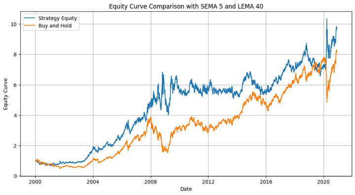
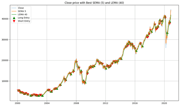
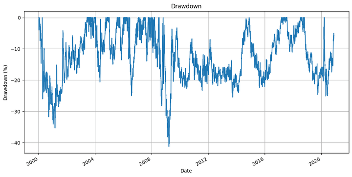
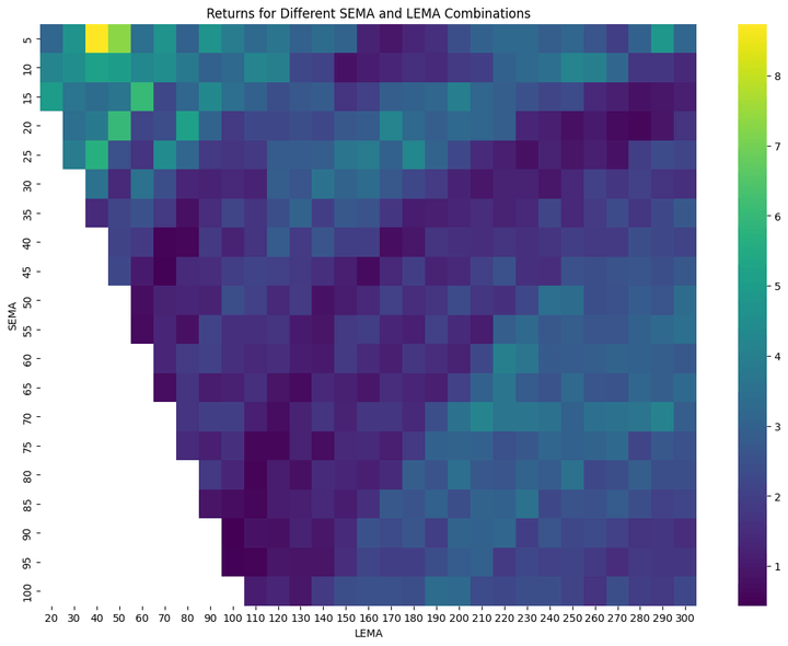
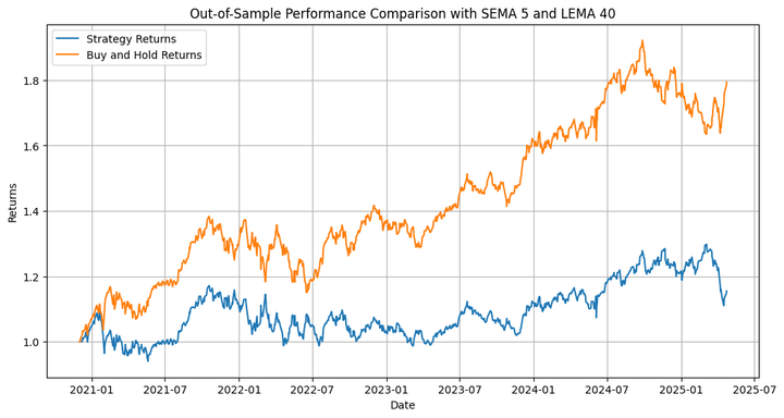

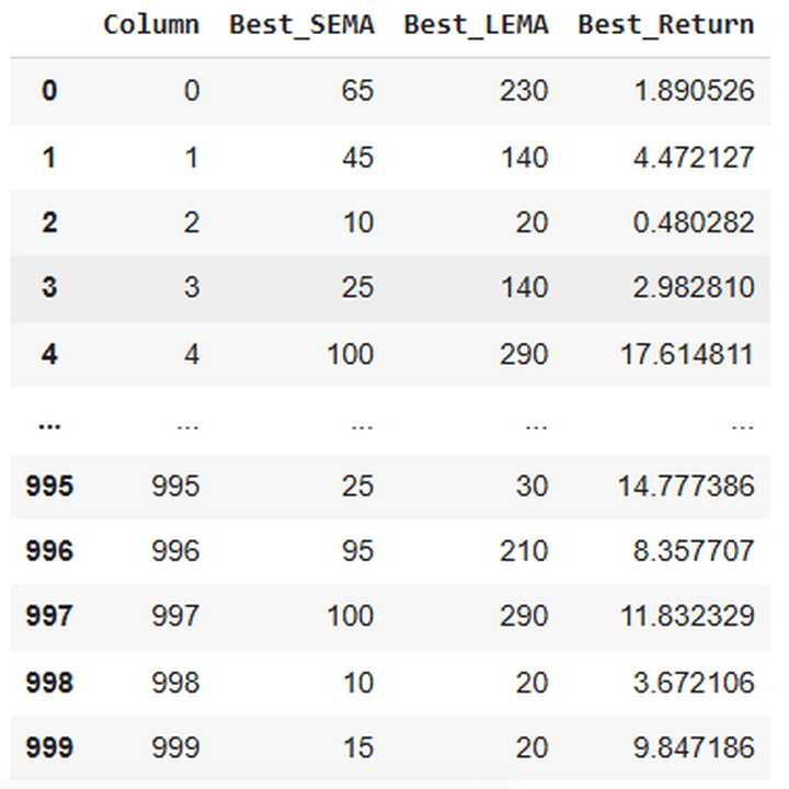
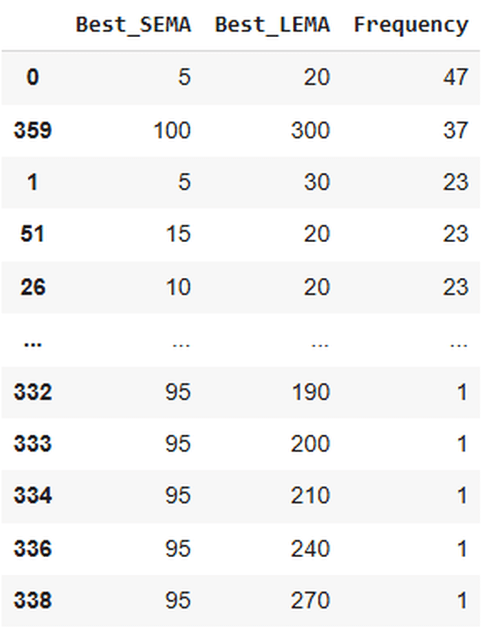
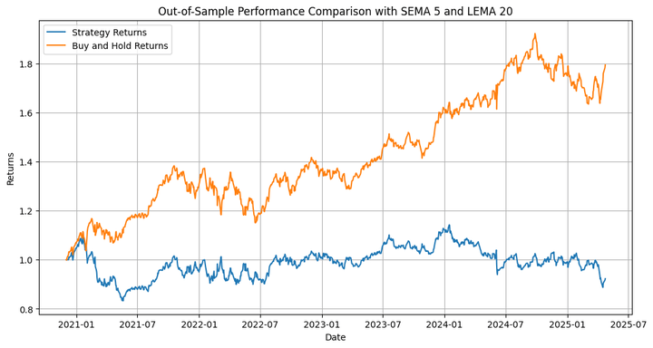
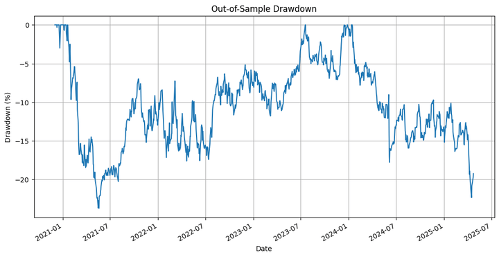
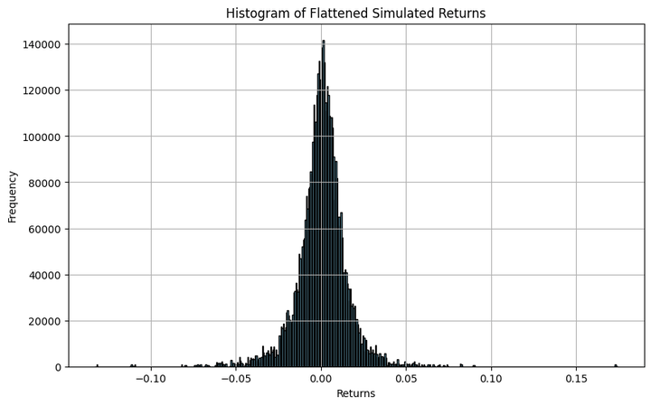
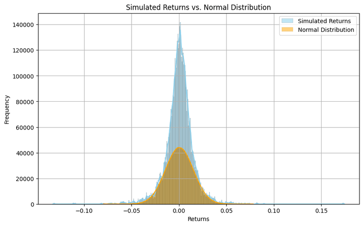


 , at every layer and for every consideration head, the mannequin produces queries
  , keys
  , and values
  . In basic Multi-Head Consideration (MHA), the computation for a single consideration head is:
 = text{softmax}left(dfrac{Q K^top}{sqrt{d_k}}right) V,")
 is the dimension of the important thing and question vectors per head. The necessity to attend to all earlier tokens for each new token pushes computational complexity from
 ") (with out caching) to
(with out caching) to ") (with caching), the place
(with caching), the place  is sequence size.
 times text{Layers} times text{Precision}")
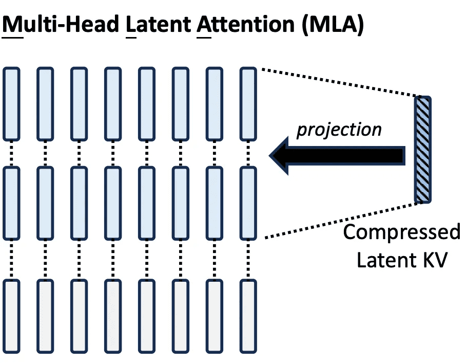
 and
and  heads, Q, Ok, V are projected as:
 is the pinnacle dimension. Autoregressive inference makes it essential to cache Ok and V for all previous steps, resulting in a big cache matrix of form
 ") per layer and per sort (Ok/V).
per layer and per sort (Ok/V).

 are considerably smaller than the unique dimensions.
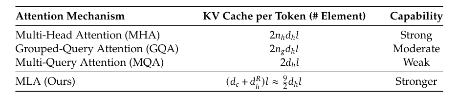
 for Ok and V,
  for Q):
 and
and  are low-dimensional latent representations,
 are decompression matrices.
V = text{softmax}left( dfrac{C_Q W^{Q_{text{up}},i} left({W^{K_{text{up}},i}}right)^top}{sqrt{d_k}}right)C_{KV} W^{V_text{up},i}")
 to
to  ,
,^top") is impartial of the enter and will be precomputed, additional saving consideration computation at inference.
is impartial of the enter and will be precomputed, additional saving consideration computation at inference.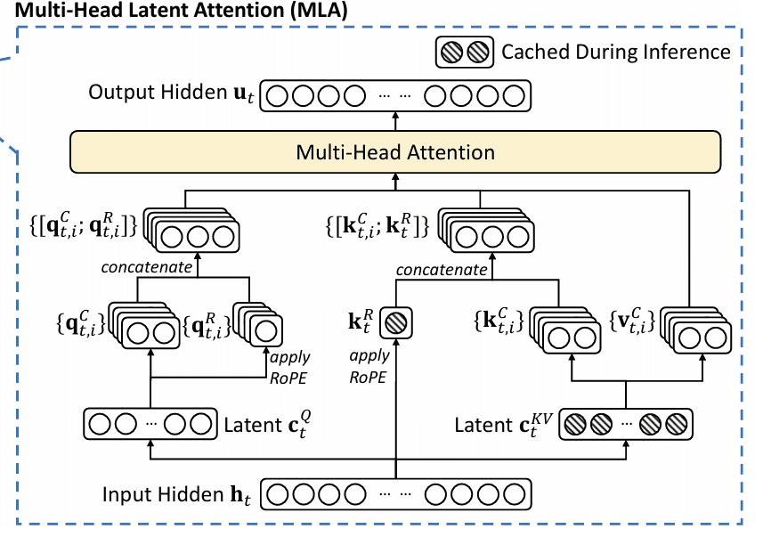
 and embedding index
  :
:}, x^{(2i+1)} right) = left( begin{bmatrix} cos(theta_{p,i}) & -sin(theta_{p,i}) sin(theta_{p,i}) & cos(theta_{p,i}) end{bmatrix} begin{bmatrix} x^{(2i)} x^{(2i+1)} end{bmatrix} right)") with
with ")
 :
:} = (c_i W_{kc}^{(s)}) oplus (x_i W_{kr} mathcal{R}_i)")
 is concatenation,
  is the low-rank latent vector,
 }") is head-specific up-projection,
is head-specific up-projection,  is projection to the RoPE subspace, and
  is the rotation matrix at place
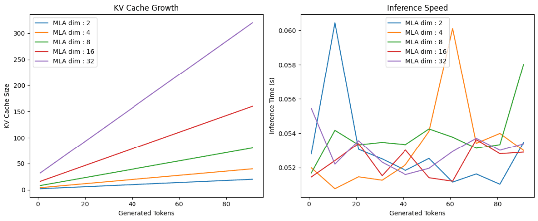


