These in want of a brilliant low cost cellphone deal could have come to the best place, seeing as Greatest Purchase is providing as much as $400 off final 12 months’s Motorola Edge as a part of an outlet and clearance sale operating via this weekend. Whereas the 2024 Edge is not going to supply peak efficiency ranges, it’s going to get the job completed for many informal customers. Plus, at $150 if you let Greatest Purchase activate it for you (or $250 in the event you activate it your self), it begins to look somewhat extra aggressive regardless of being a 2024 mannequin.
The 2024 Motorola Edge nonetheless contains the luxurious-feeling, anti-slip vegan leather-based backing, a very nice pOLED show that is simple on the eyes, and the user-friendly Whats up UI that consumers love. It comes with 256GB of storage, a 32MP entrance digicam and each an everyday rear lens and an ultrawide.
Past that, it is stated to simply recover from a full day’s value of battery life with its 5,000mAh battery, and it presents as much as 68W quick charging, making it a great decide for individuals who worth battery life.
✅Beneficial if: you are in search of a cellphone for beneath $200 or $300 that will not compromise on battery life or charging speeds; you want having a handsome show that is additionally considerably simple on the eyes; you have favored the luxurious really feel of Motorola’s anti-slip vegan leather-based backing on different telephones.
❌Skip this deal if: you are in search of a cellphone with industry-leading efficiency speeds; you worth having a cellphone with a long-term software program replace promise; you desire a cellphone with high-powered cameras and you’ve got the finances to spend somewhat extra.
The Motorola Edge lineup has supplied some respectable, lower-priced telephones over time. Nonetheless, we have nonetheless discovered a few of these worth tags somewhat costly for what you get, which is why reductions like these could also be value making the most of. Whereas lots of the finest Motorola telephones supply extra highly effective efficiency than final 12 months’s Edge, customers who do not care about having a super-fast cellphone could respect different parts of the 2024 mannequin, comparable to its long-lasting battery, 8GB of RAM, 256GB of storage, in addition to the gorgeous, 6.6-inch pOLED show, which boasts a 144Hz refresh price.
This 12 months’s Motorola Edge did embrace just a few upgrades from the 2024 mannequin, maybe most notably together with new AI options and higher cameras. For many, nonetheless, the 2024 mannequin will supply what most informal customers want, so long as you do not thoughts the truth that efficiency generally is a little sluggish at occasions.
Just a few months in the past—26 July 2025 to be exact—was the tenth anniversary of my first weblog submit. Over that point it seems I’ve written about 225 weblog posts, and an astonishing (to me) 350,000 phrases. That’s after you are taking out the code.
Free Vary Statistics is an old style weblog, with a single writer and really a lot representing the best of a “internet log” simply recording issues of curiosity to me. It’s not a complete private weblog (I by no means have posts nearly my journey, household life, and so on.), however targeted on points that one way or the other relate to statistics—starting from the summary and methodological, via to particular functions of the sort “right here’s a enjoyable chart of some fascinating historic or present information I noticed”. It’s strictly non-monetised; open to the world to learn free of charge, and can by no means make paid endorsements. I’ll go a bit into what’s saved me motivated later, however the spoiler is that, like artwork, running a blog is for my part one thing finest accomplished primarily in your personal pursuits and wishes, and if anybody else likes it that’s a bonus.
The ten years of weblog historical past hasn’t been a good one, however has had some ebbs and flows. We are able to see this on this chart of variety of weblog posts monthly over time.
Code for these charts is on the backside of the submit. Two issues value noting about this one are how I’ve turned the months with zero posts into hole circles to de-emphasise them visually whereas nonetheless together with the zeroes within the modelling; and used for the pattern line a steady single mannequin over all years as a substitute of a separate mannequin match to every year-facet, which might be the straightforward default however does probably not make sense given how time is steady and all.
The low level of submit frequency was 2021 and 2022, when life occasions bought in the best way. I used to be very busy in my day job as Chief Knowledge Scientist for Nous Group, and this additionally was pretty hands-on technical itself which diminished my motivation to jot down code out-of-hours to loosen up. I used to be additionally taking part in loads of Elite Harmful on this interval, proper up till 2024 (when the civil unrest in Noumea led me to drop that chilly turkey). Mid 2018 and mid 2022 each noticed me change jobs and international locations. In 2025 I’ve had well being challenges, however these appear to be below management and I’m entering into a greater modus vivendi with them.
The previous couple of years has seen a delicate however materials uptick in my posting frequency, and I believe that is going to proceed. I’ve bought fairly a backlog of half-finished posts to jot down about. These are on matters starting from artificial controls, to energy and p-values, to plenty of empirical stuff on the Pacific.
One factor that’s occurred over time is the posts have gotten longer and, maybe, extra thorough over time. Definitely they’re much extra more likely to be crafted over weeks and even months (or years in some circumstances), moderately than knocked out in a single Saturday morning as was once the case. Again after I wrote 45 posts in 2016—practically one every week—they have been brief, very single subject, no nice degree of element. Extra just lately I’m extra inclined to attempt to completely tease one thing out, notably when I’m studying for myself or making an attempt to consolidate my understanding of one thing. A very good instance could be my current set of posts on modelling fertility charges, which I needed to break up into two, one on the substance and one on the seize bag of issues I discovered on the best way.
Right here’s a linked scatter plot that lets us see each phrase depend and posting frequency collectively, with some very crude characterisations of attribute themes I used to be writing about on the time:
Whereas one does one’s artwork for its personal sake, there’s no denying it’s fascinating to see what different individuals learn in my weblog too. I get a modest however regular trickle of round 60 distinctive guests and 80-100 pages learn a day. That’s, modest in comparison with say Heather Armstrong’s peak numbers of about 300,000 guests a day on the peak of mummy running a blog, however fairly a couple of greater than I believed I’d get after I set out (which might have been, to be trustworthy, in spherical numbers, round zero).
At its excessive level again when Twitter roughly labored, I wrote extra regularly and was doing election forecasts, I assume I bought about 70% extra site visitors than now, nevertheless it’s exhausting to inform, with altering approaches to monitoring guests.
I used to have an automatic “hottest” itemizing however adjustments in analytics companies over the weblog’s lifetime degraded this and I’ve pulled it. However from a extra advert hoc examination utilizing partial information from some blended sources (too difficult to speak about right here), listed here are some posts which were most learn just lately:
That is fascinating and I believe might be exhibiting some exterior searches are turning up my weblog on fundamental methodological questions. This have to be dominating over social media or RSS feeds pulling in guests after I publish a brand new submit. I’m happy to say every of those posts above does certainly have one thing helpful in it—roughly outlined as that means I typically return to them myself to see what I believed. So I hope different individuals are discovering them of some use on the finish of their random internet search too.
If I had an extended collection of analytics information I’m positive my numerous election-related posts pages, and time collection modelling posts, could be within the real prime hits. At one level it appeared like a few of my comparisons of forecasting strategies have been within the required studying for some programs, they have been getting so many hits.
Weblog benchmarks
I did some cursory web analysis into weblog longevity, to see how my 10 years stands up compared. ChatGPT first assured me that analysis stated the 60-70% of blogs are deserted after one 12 months (attributed to Herring et al) and that the median life was 4 months (Mishne and de Rijke) or 50% stopped after one month (similar alleged authors).
These all sound believable! And perhaps these authors did discover that. However I can’t (with restricted time and entry, admittedly) discover them doing so. Software of intensive interrogation strategies to ChatGPT revealed that these have been issues that it thought sounded believable as issues these individuals may have written, moderately than it may truly discover actual, revealed papers that contained these numbers.
Really, ChatGPT is like an enthusiastic, immensely well-read however very unreliable analysis assistant who has had a few drinks, whose outputs ought to all be prefaced with “I appear to recollect studying or listening to someplace….” and handled with a heap of scepticism.
When it comes to actual findings I can truly supply, some analysis from again when blogs have been cool and earlier than short-form social media actually took off discovered that 1 / 4 of blogs solely final one submit. Again in 2003, apparently, “the standard weblog is written by a teenage woman who makes use of it twice a month to replace her buddies and classmates on happenings in her life.” Today, I don’t assume such individuals write blogs and even micro-blogs, however submit movies on TikTok or equal.
A 2012 research of analysis blogs—nearer in type and motivation to my very own than the extra private blogs that make (or made) up the majority of the blogosphere—discovered 84% of analysis blogs revealed below the writer’s personal identify; 86% in English; and 72% by one or two male authors. So I’m within the majority in these respects.
At round 1,500 phrases every, my weblog posts are for much longer than the common of 200-300 phrases discovered by Susan Herring and others in a 2004 research.
A lot of the analysis above is dated. Successfully it precedes the rise of video-based influencers. Quick-form video (TikTok and so on), podcasts, common video, and short-form textual content (X, Bluesky, LinkedIn and so on) appear to dominate over written blogs as of late. I’ve little interest in producing any of these items besides the short-form textual content / social media websites.
There are nonetheless apparently one million or so lively blogs, a lot of them forming a extra steady piece of infrastructure beneath the froth of those extra trendy types. That is mainly how I have interaction with Bluesky, Mastodon and LinkedIn too, when it comes to the connection with my weblog. I write within the weblog, and use the social media to publicise that writing.
Why I write my weblog
Ten years is successful, I assume. Whereas I couldn’t discover a citable supply, I’m properly ready to imagine that the majority blogs are deserted after a couple of months. So what saved me motivated to maintain writing for ten years?
My motivations have definitely advanced over time as I settled right into a rhythm of writing and publishing posts. In comparison with after I set out, I can provide a way more correct image of why I’m actually doing this:
It helps me train and lengthen my hands-on technical craft—one thing that doesn’t occur naturally within the managerial roles in my day job, however remains to be helpful for executing these roles even in a directorial and decision-making moderately than hands-on capability.
I can study issues, with the motivation for further self-discipline (I actually need to be assured I’m getting some unfamiiar factor proper if I’m going to submit it) that comes from doing so in public. Quite a lot of instances I’ve had my course corrected by optimistic engagements after posting a weblog, both on social media or within the feedback part.
Generally it’s simply enjoyable, and stress-free, to mess around with information and code. Significantly after I learn one thing fascinating and need to verify “wait, is that for actual?”. Or after I simply need to make a cool animation.
I can check out stuff we’d (or won’t) need to use at work however, for no matter purpose, wants me to offer it a go myself in a method that doesn’t slot in with my regular work tasks but could be drawn on if useful.
Generally (however not fairly often) I truly need to make an intervention within the public sphere and talk some information and concepts. How necessary this motivation is has assorted over time, and it’s by no means been notably necessary. There have been intervals after I revealed election forecasts for New Zealand that had no different equal on the time, and a few Covid modelling in Australia, the place speaking precise points was an important factor for my weblog. However these didn’t (and nearly definitely, couldn’t probably, given my power and curiosity ranges) final. Maybe the excessive level weblog submit that I actually needed individuals to learn was my publicity of Surgisphere, which made me Twitter-famous for a couple of days and was an necessary contribution to an investigation by the Guardian after which retraction of an article within the Lancet (surprisingly however gratifyingly quickly).
My day job is helped by networking, and my curiosity and abilities in information and code is one device I can use in a small method to do this. I’m definitely not into running a blog for fame (or I hope I’d do in another way and higher than I’m), however I do search to make use of my posts in a sure method to broaden and strengthen my skilled networks. I publicise my posts on Bluesky and LinkedIn, typically Fb (and till 2024 on Twitter). They’re a method of getting myself identified to area of interest audiences, and really often a method to obtain an goal for my day job by publicising one thing cool we’re doing, positions we’re recruiting, or a problem we’re involved about.
Technical stuff in regards to the weblog
After I arrange my weblog I actually, actually hated the non-data technical stuff about getting it to work, having the fonts proper, understanding how domains work, deciding on format, and so on. I needed to learn fairly a couple of blogs on arrange blogs, and vowed to myself to not turn into certainly one of them. So I’ve comparatively few posts on the again finish of my weblog. However ten years on, there may be some (small) potential curiosity in what works for me, so right here is how my weblog works below the hood:
It’s hosted on GitHub pages however has its personal area identify. This (the GitHub half) is free, and offers me loads of management over formatting, and works properly with Jekyll.
I exploit Jekyll and resisted upgrading to Hugo when it comes alongside. In issues like this, “there’s a time for change, which is when it may possibly not be resisted”. If it ain’t broke, don’t repair it.
It’s a Git repository inside a repository. The supply code is the necessary one which I work on and has a _working folder with all of the R and different technical scripts, and a _posts folder with Markdown or HTML recordsdata for the precise posts.
After I construct the positioning it seems within the _site folder of the supply code repository. _site can be a Git repository and, when it’s all good to go, I push that to the https://github.com/ellisp/ellisp.github.io repository on GitHub, which is robotically revealed on GitHub pages.
I write all of the Markdown or HTML pages by hand. I exploit HTML when issues get too difficult layout-wise for Markdown (not fairly often).
I don’t use RMarkdown or related for this weblog (knitting leads to with the code and textual content) as a result of I want to have full, guide management of the place I put a code chunk, plot or desk. And my inventive course of may be very a lot “work on the evaluation” after which “write it up”, which is properly supported by having a separate R script with the evaluation and a Mardown or HTML file with the write-up.
I created and use the frs R bundle with a couple of supporting features, most necessary of which is the svg_png() operate. It makes use of the strategy described on this submit. It helps SVG recordsdata look good with Google fonts and dealing throughout platforms. It additionally saves near-identical PNG and SVG variations of pictures, so I can have PNG fall-backs for browsers that don’t present SVGs (this was an actual concern 10 years in the past, I don’t find out about now).
There are some issues like syntax highlighting, the area identify, hyperlink to Disqus for feedback part, that concerned a bunch of mucking round that I’m happy to say I’ve forgotten utterly what I needed to do.
Yeah, weblog to reside, don’t reside to weblog. That’s true on the whole, however by no means extra so than in fascinated about the stuff that makes it potential to weblog.
Phrase depend code
Right here’s the code that produced the charts proven earlier on this submit:
library(tidyverse)library(stylo)# for delete.markuplibrary(glue)library(ggtext)#---------------Import and course of weblog posts-------------blog_names<-checklist.recordsdata("../_posts",full.names=TRUE)blogs<-tibble()for(iin1:size(blog_names)){blogs[i,"full"]<-paste(readLines(blog_names[i]),collapse=" ")blogs[i,"filename"]<-gsub("../_posts/","",blog_names[i],fastened=TRUE)}blogs<-blogs|>mutate(no_jekyll=gsub("{% spotlight R.*?%}.*?{% endhighlight %}"," ",full),txt="")# delete markup solely works on one string at a time, appears best to do it in a loop:for(iin1:nrow(blogs)){blogs[i,]$txt<-delete.markup(blogs[i,]$no_jekyll,markup.kind="html")}# a couple of extra fundamental stats per weblog submit:blogs<-blogs|>mutate(word_count=stringi::stri_count_words(txt),word_count_with_tags=stringi::stri_count_words(no_jekyll),date=as.Date(str_extract(filename,"^[0-9]*-[0-9]*-[0-9]*")),month=month(date),12 months=12 months(date))#---------------Minimal anaylsis----------------# Abstract aggregatesblog_sum<-blogs|>summarise(number_blogs=n(),words_with_tabs=sum(word_count_with_tags),total_words=sum(word_count),mean_words=imply(word_count),median_words=median(word_count),max_words=max(word_count),min_words=min(word_count))# Shortest weblog (seems to be one simply saying a piece shiny app):blogs|>organize(word_count)|>slice(1)|>pull(txt)#------------------Graphics to be used in blog-------------------------the_caption<-"Supply: https://freerangestats.information"# Time collection plot exhibiting variety of posts by month:d1<-blogs|>group_by(12 months,month)|>summarise(number_blogs=n())|>ungroup()|>full(12 months,month,fill=checklist(number_blogs=0))|># take away October, November, December in 2025 (as time of writing is September 2025):filter(!(12 months==2025&month%in%10:12))|># take away months weblog didn't exist:filter(!(12 months==2015&month%in%1:6))|>group_by(12 months)|>mutate(year_lab=glue("{12 months}: {sum(number_blogs)} posts"),is_zero=ifelse(number_blogs==0,"Zero","NotZero"))# mannequin a clean curve to the entire information set (don't need)# to do that with geom_smooth within the plot as then it has# break yearly:mod<-loess(number_blogs~I(12 months+month/12),information=d1,span=0.15)d1$fitted<-predict(mod)# draw time collection plot of variety of blogs:d1|>ggplot(aes(x=month,y=number_blogs))+facet_wrap(~year_lab)+geom_line(aes(y=fitted),color="grey80")+geom_point(color="steelblue",measurement=2.5,aes(form=is_zero))+expand_limits(y=0)+scale_x_continuous(breaks=1:12,labels=month.abb)+scale_shape_manual(values=c("Zero"=1,"NotZero"=19))+theme(panel.grid.minor=element_blank(),axis.textual content.x=element_text(angle=45,hjust=1),legend.place="none")+labs(x="",y="Variety of weblog posts",title="Ten years of Free Vary Statistics running a blog",subtitle=glue("{nrow(blogs)} posts and {comma(blog_sum$total_words)} phrases, in simply over ten years."),caption=the_caption)# Linked scatter plot evaluating common phrase depend to variety of posts:blogs|>mutate(number_months=case_when(12 months==2015~6,12 months==2025~8.5,TRUE~12))|>group_by(12 months,number_months)|>summarise(avg_word_count=imply(word_count,tr=0.1),number_blogs=n())|>ungroup()|>mutate(blogs_per_month=number_blogs/number_months)|>ggplot(aes(x=blogs_per_month,y=avg_word_count,label=12 months))+geom_path(color="grey80")+geom_text(color="grey50")+scale_y_continuous(label=comma)+expand_limits(x=4.5)+annotate("textual content",fontface="italic",hjust=0,color="darkblue",x=c(4,3.4,2.1),y=c(1165,1350,1880),label=c("Time collection","Elections","Covid"))+# add day jobsannotate("textual content",fontface="italic",hjust=0,color="brown",x=c(3.1,2.5,0,1.1),y=c(1130,1675,1420,1330),label=c("NZ economics","Marketing consultant","Chief Knowledge Scientist","Pacific"))+labs(x="Weblog posts monthly",y="Common phrases per weblog submit",title="Ten years of Free Vary Statistics running a blog",subtitle="Annotated with necessary (however not essentially dominant) themes and day-jobs for various phases.",caption=the_caption)+theme(plot.subtitle=element_markdown())
A brand new personal moon lander may take flight just some years from now.
Impulse House — a industrial house firm based by Tom Mueller, the primary worker the billionaire Elon Musk ever employed at SpaceX — introduced on Tuesday (Oct. 14) that it plans to construct a robotic moon lander to assist open the lunar frontier.
“To echo President John F. Kennedy, going to the moon is tough. However we all know that we now have a number of the brightest minds in aerospace engineering right here at Impulse, who push the boundaries of innovation ahead day-after-day,” Mueller wrote in a weblog submit on Tuesday that laid out Impulse’s lunar imaginative and prescient. “We’re assured in our means to resolve expertise’s hardest challenges and excited to proceed accelerating our future past Earth.”
Impulse House may launch its first lunar touchdown mission as quickly as 2028. (Picture credit score: Impulse House)
Impulse House, which Mueller based in 2021, focuses on in-space transportation — getting spacecraft the place they should go after they launch into the ultimate frontier.
The corporate already operates a dishwasher-sized house tug referred to as Mira, which reached house for the primary time on SpaceX’s Transporter 9 rideshare mission in November 2023. Impulse can also be engaged on a “kick stage” referred to as Helios, which is designed to ship massive payloads from low Earth orbit to higher-energy locations like geostationary orbit and Earth-moon house. Helios is scheduled to make its spaceflight debut in late 2026.
Impulse’s moon plans contain that Helios kick stage and a brand new lunar lander, which the corporate will construct in-house. The duo will launch collectively on a typical medium- or heavy-lift rocket, in accordance with Mueller’s weblog submit.
“As soon as Helios and the lander are deployed in low Earth orbit (LEO), Helios serves as a cruise stage, transporting the lander to low lunar orbit inside one week,” he wrote. “The lunar lander then separates from Helios and descends to the floor of the moon. By benefiting from Helios’ excessive delta-v capabilities, this mission structure would not require in-space refueling.”
Breaking house information, the newest updates on rocket launches, skywatching occasions and extra!
Every Helios-lander mission will be capable of put 3 tons of payload down on the moon, Mueller stated. The primary such supply may happen as quickly as 2028, he added.
A variety of personal lunar landers are already flying or in improvement. For instance, Houston firm Intuitive Machines has launched its Nova-C spacecraft to the moon twice already, and Tokyo-based ispace has achieved the identical with its Hakuto-R craft.
Peregrine, a spacecraft constructed by Pittsburgh-based Astrobotic, has one flight underneath its belt, as does Firefly Aerospace’s Blue Ghost. (Blue Ghost is the one one with a totally profitable mission to its identify; Nova-C tipped over shortly after touchdown on each of its moon flights, Hakuto-R crashed onerous into the lunar floor twice, and Peregrine did not make it out of Earth orbit.)
The above are all comparatively small robotic landers, however there are greater, crew-capable moon craft in improvement as nicely. As an example, NASA has tapped SpaceX’s Starship and Blue Origin’s Blue Moon automobile to get its Artemis astronauts down safely on the lunar floor.
Impulse House goals to bridge the hole between these two lander classes, providing an economical approach to get midsize payloads down on the moon, in accordance with Mueller.
“We’d like landers able to near-term, multi-ton cargo deliveries with a view to quickly construct out a sustainable lunar presence,” he wrote. “These kinds of deliveries may embrace issues like a lunar terrain automobile, rovers, communication relay programs, energy mills and habitation modules.”
Impulse House has already began engaged on the moon lander’s engine, which can “use a nitrous and ethane bipropellant — the identical mixture used efficiently in house on Mira,” Mueller wrote.
And he reminded readers that Impulse took Mira from a mere design on paper to a functioning spacecraft in Earth orbit in lower than 15 months.
“We’re assured in our means to ship this answer due to our robust observe file of fast success,” Mueller wrote of his firm’s moon plans.
T. Y. V. de Lima Cavalcanti, M. R. Pereira, S. O. de Paula, and R. F. de O. Franca, “A evaluation on Chikungunya virus epidemiology, pathogenesis and present vaccine improvement,” Viruses, vol. 14, no. 5, p. 969, 2022.
[3]
H. Z. W. Van Bortel Bertrand Sudre, “Chikungunya: Its Historical past in Africa and Asia and Its Unfold to New Areas in 2013–2014,” https://educational.oup.com/, 15-Dec-2016. [Online]. Obtainable: https://educational.oup.com/jid/article/214/suppl_5/S436/2632642. [Accessed: 31-Jul-2025].
[4]
M. Delrieu et al., “Temperature and transmission of chikungunya, dengue, and Zika viruses: A scientific evaluation of experimental research on Aedes aegypti and Aedes albopictus,” Curr. Res. Parasitol. Vector Borne Dis., vol. 4, p. 100139, 2023.
D. Mavalankar, P. Shastri, T. Bandyopadhyay, J. Parmar, and Ok. V. Ramani, “Elevated mortality fee related to chikungunya epidemic, Ahmedabad, India,” Emerg. Infect. Dis., vol. 14, no. 3, pp. 412–415, 2008.
L. A. Silva and T. S. Dermody, “Chikungunya virus: epidemiology, replication, illness mechanisms, and potential intervention methods,” J. Clin. Make investments., vol. 127, no. 3, pp. 737–749, 2017.
[10]
W H Ng , Ok Amaral , E Javelle , S Mahalingam, “Continual chikungunya illness (CCD): medical insights, immunopathogenesis and therapeutic views,” https://educational.oup.com/, 20-Feb-2024. [Online]. Obtainable: https://educational.oup.com/qjmed/article/117/7/489/7611656. [Accessed: 31-Jul-2025].
[11]
J. Ok. Amaral, C. O. Bingham third, P. C. Taylor, L. M. Vilá, M. E. Weinblatt, and R. T. Schoen, “Pathogenesis of persistent chikungunya arthritis: Resemblances and hyperlinks with rheumatoid arthritis,” Journey Med. Infect. Dis., vol. 52, no. 102534, p. 102534, 2023.
[12]
M. van Aalst Charlotte Marieke Nelen Abraham Goorhuis Cornelis Stijnis Martin Peter Grobusch, “Lengthy-term sequelae of chikungunya virus illness: A scientific evaluation,” Sciencedirect.com, 20-Feb-2017. [Online]. Obtainable: https://www.sciencedirect.com/science/article/abs/pii/S1477893917300042. [Accessed: 31-Jul-2025].
[13]
CDC, “Therapy and prevention of Chikungunya virus illness,” Chikungunya Virus, 16-Could-2025. [Online]. Obtainable: https://www.cdc.gov/chikungunya/hcp/treatment-prevention/index.html. [Accessed: 31-Jul-2025].
[14]
“FDA Approves First Vaccine to Forestall Illness Brought on by Chikungunya Virus,” Fda.gov, 09-Nov-2023. [Online]. Obtainable: https://www.fda.gov/news-events/press-announcements/fda-approves-first-vaccine-prevent-disease-caused-chikungunya-virus. [Accessed: 31-Jul-2025].
State area fashions are a strong instrument for analyzing time collection information, particularly while you need to estimate unobserved parts like traits or cycles. However historically, organising these fashions—even for one thing as frequent as ARIMA—will be tedious.
The GAUSS arimaSS perform, accessible within the Time Collection MT 4.0 library, enables you to estimate state area ARIMA fashions with out manually constructing the total state area construction. It’s a cleaner, sooner, and extra dependable method to work with ARIMA fashions.
On this submit, we’ll revisit our inflation modeling instance utilizing up to date information from the Federal Reserve Financial Information (FRED) database. Alongside the way in which, we’ll reveal how arimaSS works, the way it simplifies the modeling course of, and the way straightforward it’s to generate forecasts out of your outcomes.
Why use arimaSS in TSMT?
In our earlier state-space inflation instance, we manually arrange the state area mannequin. This course of required a strong understanding of state area modeling, particularly:
Establishing the system matrices.
Initializing state vectors.
Managing mannequin dynamics.
Specifying parameter beginning values.
Compared, the arimaSS perform handles all of this setup mechanically. It internally constructs the suitable mannequin construction and runs the Kalman filter utilizing commonplace ARIMA specs.
Total, the arimaSS perform offers:
Simplified syntax: No must manually outline matrices or system dynamics. This not solely saves time but in addition reduces the possibility of errors or mannequin misspecification.
Extra strong estimates: Behind-the-scenes enhancements, corresponding to enhanced covariance computations and stationarity enforcement, result in extra correct and steady parameter estimates.
Compatibility with forecasting instruments: The arimaSS output construction integrates straight with TSMT instruments for computing and plotting forecasts.
The arimaSS Process
The arimaSS process has two required inputs:
A time collection dataset.
The AR order.
It additionally permits 4 elective inputs for mannequin customization:
The order of differencing.
The transferring common order.
An indicator controlling whether or not a continuing is included within the mannequin.
An indicator controlling whether or not a pattern is included within the the mannequin.
Normal Utilization
aOut = arimaSS(y, p [, d, q, trend, const]);
Y
Tx1 or Tx2 time collection information. Might embody date variable, which shall be faraway from the info matrix and isn’t included within the mannequin as a regressor.
p
Scalar, the variety of autoregressive lags included within the mannequin.
d
Optionally available, scalar, the order of differencing. Default = 0.
q
Optionally available, scalar, the transferring common order. Default = 0.
pattern
Optionally available, scalar, an indicator variable to incorporate a pattern within the mannequin. Set to 1 to incorporate pattern, 0 in any other case. Default = 0.
const
Optionally available, an indicator variable to incorporate a continuing within the mannequin. Set to 1 to incorporate fixed, 0 in any other case. Default = 1.
All returns are saved in an arimaOut construction, together with:
Estimated parameters.
Mannequin diagnostics and abstract statistics.
Mannequin description.
The entire contents of the arimaOut construction embody:
Member
Description
amo.aic
Akaike Data Criterion worth.
amo.b
Estimated mannequin coefficients (Kx1 vector).
amo.e
Residuals from the fitted mannequin (Nx1 vector).
amo.ll
Log-likelihood worth of the mannequin.
amo.sbc
Schwarz Bayesian Criterion worth.
amo.lrs
Probability Ratio Statistic vector (Lx1).
amo.vcb
Covariance matrix of estimated coefficients (KxK).
amo.mse
Imply squared error of the residuals.
amo.sse
Sum of squared errors.
amo.ssy
Complete sum of squares of the dependent variable.
amo.rstl
Occasion of kalmanResult construction containing Kalman filter outcomes.
amo.tsmtDesc
Occasion of tsmtModelDesc construction with mannequin description particulars.
amo.sumStats
Occasion of tsmtSummaryStats construction containing abstract statistics.
Instance: Modeling Inflation
At the moment, we’ll use a easy, albeit naive, mannequin of inflation. This mannequin relies on a CPI inflation index created from the FRED CPIAUCNS month-to-month dataset.
To start, we’ll load and put together our information straight from the FRED database.
Pull the constantly compounded annual fee of change from FRED.
Embrace information ranging from January 1971 (1971m1).
// Set commentary begin date
fred_params = fred_set("observation_start", "1971-01-01");

// Specify models to be
// steady compounded annual
// fee of change
fred_params = fred_set("models", "cca");

// Specify collection to drag
collection = "CPIAUCNS";

// Pull information from FRED
cpi_data = fred_load(collection, fred_params);

// Preview information
head(cpi_data);
To additional preview our information, let’s create a fast plot of the inflation collection utilizing the plotXY process and a system string:
plotXY(cpi_data, "CPIAUCNS~date");
For enjoyable, let’s add a reference line to visualise the Fed’s long-run common inflation goal of two%:
// Add inflation goal line at 2%
plotAddHLine(2);
As one remaining visualization, let us take a look at the 5 12 months (60 month) transferring common line:
// Compute transferring common
ma_5yr = movingAve(cpi_data[., "CPIAUCNS"], 60);

// Add to time collection plot
plotXY(cpi_data[., "date"], ma_5yr);

// Add inflation targetting line at 2%
plotAddHLine(2);
The transferring common plot highlights long-term traits, filtering out short-term fluctuations and noise:
The Disinflation Period: (app. 1980-1993): This era is marked by the steep decline in inflation from the double-digit highs of the early Nineteen Eighties to round 3% by the early Nineties, an end result of aggressive financial coverage by the Federal Reserve.
The ‘Nice Moderation’ (mid-Nineties- mid-2000s): Inflation remained comparatively steady and low, hovering close to the Fed’s 2% goal, marked right here with a horizontal line for reference.
Publish-GFC stagnation (2008-2020): After the 2008 International Monetary Disaster, inflation trended even decrease, with the 5-year common dipping beneath 2% for an prolonged interval, reflecting sluggish demand and protracted slack.
Latest surge: The sharp rise starting round 2021 displays the post-pandemic spike in inflation, pushing the 5-year common above 3% for the primary time in over a decade.
We’ll make one remaining transformation earlier than estimation by changing the “CPIAUCNS” values from percentages to decimals.
Be aware: The fred_load process requires a legitimate API key. To obtain information straight from FRED into GAUSS, it’s essential to acquire an API key from FRED and set it in GAUSS.For extra particulars on importing information from FRED, see our earlier weblog submit, Importing FRED Information to GAUSS.
ARIMA Estimation
Now that we’ve loaded our information, we’re able to estimate our mannequin utilizing arimaSS. We’ll begin with a easy AR(2) mannequin. Primarily based on the sooner visualization, it’s affordable to incorporate a continuing however exclude a pattern, so we’ll use the default settings for these choices.
name arimaSS(cpi_data, 2);
There are a number of useful issues to notice about this:
We didn’t must take away the date vector from cpi_data earlier than passing it to arimaSS. Most TSMT features assist you to embody a date vector along with your time collection. Actually, that is really helpful, GAUSS will mechanically detect and use the date vector to generate extra informative outcomes stories.
On this instance, we’re not storing the output. As a substitute, we’re printing it on to the display utilizing the name key phrase.
As a result of that is strictly an AR mannequin and we’re utilizing the default deterministic parts, we solely want two inputs: the info and the AR order.
An in depth outcomes report is printed to display:
There are some attention-grabbing observations from our outcomes:
The estimated fixed is statistically important and equal to 0.038 (3.8%). That is greater than the Fed’s long-run inflation goal of two%, however not by a lot. It’s additionally vital to notice that our dataset begins nicely earlier than the period of formal Fed inflation focusing on.
All coefficients are statistically important besides for the CPIAUCNS L(2) coefficient.
The desk header contains the timespan of our information. This was mechanically detected as a result of we included a date vector with our enter. If no date vector is included, the timespan shall be reported as unknown.
The arimaSS process doesn’t at present present built-in optimum lag choice. Nonetheless, we will write a easy for loop and use an array of buildings to establish the perfect lag size.
Our purpose is to pick the mannequin with the bottom AIC, permitting for a most of 6 lags.
Two instruments will assist us with this activity:
An array of buildings to retailer the outcomes from every mannequin.
A vector to retailer the AIC values from every mannequin.
// Set most lags
maxlags = 6;

// Declare a single array
struct arimamtOut amo;

// Reshape to create construction array
amo = reshape(amo, maxlags, 1);

// AIC storage vector
aic_vector = zeros(maxlags, 1);
Subsequent, we’ll loop by means of our fashions. In every iteration, we are going to:
Retailer the ends in a separate arimamtOut construction.
Extract the AIC and retailer it in our AIC vector.
Regulate the pattern dimension so that every lag choice iteration makes use of the identical variety of observations.
// Loop by means of lag prospects
for i(1, maxlags, 1);
    // Trim information to implement pattern
    // dimension consistency
    y_i = trimr(cpi_data, maxlags-i, 0);

    // Estimate the present
    // AR(i) mannequin
    amo[i] = arimaSS(y_i, i);

    // Retailer AIC for straightforward comparability
    aic_vector[i] = amo[i].aic;
endfor;
Lastly, we are going to use the minindc process to seek out the index of the minimal AIC:
// Optimum lag is the same as location
// of minimal AIC
opt_lag = minindc(aic_vector);

// Print optimum lags
print "Optimum lags:"; opt_lag;

// Choose the ultimate output construction
struct arimamtOut amo_final;
amo_final = amo[opt_lag];
The optimum lags based mostly on the minimal AIC is 8, yielding the next outcomes:
It’s value noting that solely the coefficients for the first, 4th, and seventh lags are statistically important. This implies {that a} mannequin together with solely these lags could also be extra applicable.
Conclusion
The arimaSS perform affords a streamlined method to estimating ARIMA fashions in state area kind, eliminating the necessity for handbook specification of system matrices and preliminary values. This makes it simpler to discover fashions, experiment with lag buildings, and generate forecasts, particularly for customers who might not be deeply acquainted with state area modeling.
Eric( Director of Purposes and Coaching at Aptech Programs, Inc. )
Eric has been working to construct, distribute, and strengthen the GAUSS universe since 2012. He’s an economist expert in information evaluation and software program growth. He has earned a B.A. and MSc in economics and engineering and has over 18 years of mixed business and tutorial expertise in information evaluation and analysis.
This e-book is for intermediate Swift builders who already know the fundamentals of Swift and need to deepen their data and understanding of the language.
Protocols & Generics
Numerics & Ranges
Sequences & Collections
Unsafe
Purposeful Reactive Programming
Goal-C Interoperability
Library & API Design
Grasp the Swift language with the Skilled Swift e-book!
Swift is a wealthy language with a plethora of options to supply. Studying the official documentation or entry-level books is necessary, however it’s not sufficient to know the true energy of the language.
Skilled Swift is right here to assist, by displaying…
Grasp the Swift language with the Skilled Swift e-book!
Swift is a wealthy language with a plethora of options to supply. Studying the official documentation or entry-level books is necessary, however it’s not sufficient to know the true energy of the language.
Skilled Swift is right here to assist, by displaying you how one can harness the total energy of Swift. You’ll study superior usages of protocols, generics, purposeful reactive programming, API design and extra.
This part tells you a number of issues that you must know earlier than you get began, comparable to what you’ll want for {hardware} and software program, the place to search out the undertaking recordsdata for this e-book, and extra.
The primary part of this e-book covers the fundamental constructing blocks of the Swift language: The kind system (enums, structs and courses), Protocols and Generics. We’ll begin with a quick refresher of every matter after which leap proper into the behind-the-scenes implementations.
The content material of this part will expose the inside workings of the kind system, in addition to get you intimately aware of protocols and generics.
Welcome to Skilled Swift. On this chapter, you’ll study a number of the motivations behind creating the Swift language, take a brief however deep dive into the Swift toolchain stream and have a look at Swift. You’ll develop a easy language characteristic, ifelse, to discover a number of the services Swift presents for creating highly effective, expressive abstractions.
Varieties are important to constructing Swift packages. The Swift compiler kind checks your code to confirm correctness, guarantee security and allow better optimization. You’ll achieve expertise concerning the completely different nominal sorts and mutation with a number of small examples. You’ll additionally implement mutable worth semantics for a QuadTree kind utilizing copy-on-write dynamic storage.
On this chapter you may undergo a quick refresher on the fundamentals of protocols in addition to a few of their extra hardly ever used options.
You’ll additionally study widespread patterns that use protocols in addition to some helpful gotchas and edge instances to bear in mind.
On this chapter, you may get intimately aware of generics by persevering with to work on the networking library you began within the earlier chapter. You will learn to write generic features, courses and structs; how one can use protocols with related sorts; what kind erasure is and how one can put all that collectively to make a coherent API.
This sections covers the bottom layer of writing Swift packages: Numerics, Ranges, Strings, Sequences, Collections, Codable and the much less apparent, however essential matter – Unsafe.
As you’d anticipate from a complicated e-book, we don’t solely clarify these subjects, but additionally examine how they’re constructed, how they’re represented, and how one can use them successfully.
Swift is a platform-agnostic, general-purpose programming language that helps varied numeric sorts with differing area, vary, accuracy and efficiency traits. Constructing two apps (BitViewer and Mandlebrot), you’ll see how Swift simplifies programming with protocols and generics. You’ll additionally have a look at vary sorts and the way operators and generics as soon as once more come to the rescue in implementing these language options.
Sequence, Assortment and associated protocols kind the spine of the usual library for sorts like Array, Dictionary and Set. You’ll see how these protocols assist you to write generic algorithms that function throughout households of collections. The usual library presents some ways to rapidly construct customized sequences and collections. You’ll use these to construct a number of examples together with a customized mutable assortment to implement Conway’s Sport of Life. You’ll additionally create a chunking algorithm that can be utilized with any assortment kind.
The right implementation of a string kind in Swift has been a controversial matter for fairly a while. The design is a fragile stability between Unicode correctness, encoding agnosticism, ease-of-use and high-performance. Nearly each main launch of Swift has refined the String kind to the superior design we’ve in the present day. You’ll study how one can most successfully use strings, what they are surely, how they work and the way they’re represented.
When growing your app, you’ll typically take care of a myriad of information fashions and varied exterior items of information that you just’ll need to signify as information fashions in your app.
On this chapter, you’ll rapidly flick through the fundamentals of Codable, after which give attention to the superior supplies down the darkish corners of codable sorts.
Swift is a memory-safe and type-safe language. In some instances, you may want your code to be extraordinarily optimized, during which case the tiny overhead added by the protection checks from Swift could be too costly. You could be coping with an enormous stream of real-time information, manipulating massive recordsdata or different massive operations that take care of massive information.
On this chapter you may learn to use unsafe Swift to straight entry reminiscence via quite a lot of pointer sorts and how one can work together with the reminiscence system straight.
The ultimate part of this e-book covers superior strategies to super-charge your Swift powers, and use all of what Swift has to supply.
We’ll cowl subjects like Larger order features, Purposeful reactive programming, Goal-C interoperability, utilizing Instrumentation, and API design.
Larger-order features can simplify your code considerably by making it extra readable, loads shorter and simpler to reuse. You will study what are increased order features, what’s currying and study examples of how they’re utilized in the usual library.
On this chapter you may study an important and refined ideas of purposeful reactive programming and how one can apply these ideas to your apps.
Prefer it or not, Goal-C remains to be a closely used language in legacy codebases and apps which have been in manufacturing for a few years. In your personal apps, you’ll typically have a large Goal-C codebase that simply doesn’t really feel at house inside your Swift code or need to use a few of your shiny new Swift code in your Goal-C code.
On this chapter, you may learn to create a healthful expertise for customers of each the Goal-C and Swift parts of your codebase in a means that feels as if it had been designed for both.
Being an amazing iOS software program engineer is not solely about being a grandmaster of the Swift language. It is also about realizing which instruments the platform places at your disposal, how one can use them to sharpen your abilities and how one can establish areas of enchancment in your code.
On this chapter you may study superior options of the Devices app, and how one can use it to enhance your code.
Discover a number of subjects to boost your skillset and instinct for designing nice APIs.
Matters like Documentation, Encapsulation, versioning, and several other highly effective language options.
This put up, supposed to be the primary in a collection associated to discrete diffusion fashions, has been sitting in my drafts for months. I believed that Google’s launch of Gemini Diffusion could be a superb event to lastly publish it.
Whereas discrete time Markov chains – sequences of random variables through which the previous and future are impartial given the current – are moderately well-known in machine studying, fewer individuals ever come throughout their steady cousins. On condition that these fashions function in work on discrete diffusion fashions (see e.g. Lou et al, 2023, Sahoo et al, 2024, Shi et al, 2024, clearly not a whole listing), I believed it might be a great way to get again to running a blog by writing about these fashions – and who is aware of, perhaps keep it up writing a collection about discrete diffusion. For now, the objective of this put up is that will help you construct some key instinct about how continuous-time MCs work.
A Markov chain is a stochastic course of (infinite assortment of random variables listed by time $t$) outlined by two properties:
the random variables take discrete values (we name them states), and
the method is memory-less: What occurs to the method sooner or later solely relies on the state it’s in in the mean time. Mathematically, $X_{u} perp X_s vert X_t$ for all $s > t > u$, the place $perp$ denotes conditional independence.
We differentiate Markov chains on values the index $t$ can take: if $t$ is an integer, we name it a discrete-time Markov chain, and when $t$ is actual, we name the method a continuous-time Markov chain.
Discrete Markov chains are totally described by a set of state transition matrices $P_t = [P(X_{t+1} = ivert X_{t}=j)]{i,j}$. Observe that this matrix $P_t$ is listed by the point $t$, as it may possibly, on the whole, change over time. If $P_t = P$ is fixed, we name the Markov chain homogeneous.
Steady time homogeneous chains
To increase the notion of MC to steady time, we’re first going to develop an alternate mannequin of a discrete chains, by contemplating ready occasions in a homogeneous discrete-time Markov chain. Ready occasions are the time the chain spends in the identical state earlier than transitioning to a different state. If the MC is homogeneous, then in each timestep it has a hard and fast likelihood $p_{i,i}$ of staying there. The ready time due to this fact follows a geometric distribution with parameter $p_{i,i}$.
The geometric distribution is the one discrete distribution with the memory-less property, said as $mathbb{P}[T=s+tvert T>s] = mathbb{P}[T = t]$. What this implies is: if you’re at time s, and you recognize the occasion hasn’t occurred but, the distribution of the remaining ready time is identical, no matter how lengthy you’ve got been ready. It seems, the geometric distribution is the one discrete distribution with this property.
With this statement, we will alternatively describe a homogeneous discrete-time Markov chain when it comes to ready occasions, and leap possibilities as follows. Ranging from state $i$ the Markov chain:
stays in the identical state for a time drawn from a Geometric distribution with parameter $p_{i,i}$
when the ready time expires, we pattern a brand new state $i neq j$ with likelihood $frac{p_{i,j}}{sum_{kneq i} p_{i,okay}}$
In different phrases, we have now decomposed the outline of the Markov chain when it comes to when the subsequent leap occurs, and the way the state modifications when the leap occurs. On this illustration, if we wish one thing like a Markov chain in steady time, we will try this by permitting the ready time to take actual, not simply integer, values. We will do that by changing the geometric distribution by a steady likelihood distribution. To protect the Markov property, nevertheless, it will be important that we protect the memoryless property $mathbb{P}[T=s+tvert T>s] = mathbb{P}[T = t]$. There is just one such steady distribution: the exponential distribution. A homogeneneous continuous-time Markov chain is thus described as follows. Ranging from state $i$ at time $t$:
keep in the identical state for a time drawn from an exponential distribution with some parameter $lambda_{i,i}$
when the ready time expires, pattern a brand new state $i neq j$ with likelihood $frac{lambda_{i,j}}{sum_{kneq i} lambda_{i,okay}}$
Discover that I launched a brand new set of parameters $lambda_{i,j}$ which now changed the transition possibilities $p_{i,j}$. These not should be likelihood distributions, they simply should be all optimistic actual values. The matrix containing these parameters will likely be referred to as the speed matrix, which I’ll denote by $Lambda$, however I will notice that in current machine studying papers, they usually use the notation $Q$ for the speed matrix.
Non-homogeneous Markov chains and level processes
The above description solely actually works for homogeneous Markov chains, through which the ready time distribution doesn’t change over time. When the transition possibilities can change over time, the wait time can not be described as exponential, and it is truly not so trivial to generalise to steady time on this method. To do this, we want one more various view on how Markov chains work: we as a substitute contemplate their relationship to level processes.
Level processes
Think about the next state of affairs which is able to illustrate the connection between the discrete uniform, the Bernoulli, the binomial and the geometric distributions.
The Easter Bunny is hiding eggs in 50 meter lengthy (one dimensional) backyard. In each 1 meter phase he hides at most one egg. He needs to guarantee that on common, there’s a 10% probability of an egg in every 1 meter phase, and he additionally needs the eggs to seem random.
Bunny is contemplating a number of other ways of reaching this:
Course of 1: Bunny steps from sq. to sq.. At each sq., he hides an egg with likelihood 0.1, and passes to the subsequent sq..
bernoulli = partial(numpy.random.binomial, n=1)
backyard = ['_']*50

for i in vary(50):
  if bernoulli(0.1)
    backyard[i] = '🥚'

print(''.be a part of(backyard))

>>> __________🥚__🥚______🥚_🥚__________________🥚________
Simulating the egg-hiding course of utilizing Bernoulli distributions
Course of 2: At every step Bunny attracts a random non-negative integer $T$ from a Geometric distribution with parameter 0.1. He then strikes T cells to the appropriate. If he’s nonetheless inside bounds of the backyard, he hides an egg the place he’s, and repeats the method till he’s out of bounds.
backyard = ['_']*50
bunny_pos = -1

whereas bunny_pos<50:
  bunny_pos += geometric(0.1)
  if bunny_pos<50:
    backyard[bunny_pos] = '🥚'

print(''.be a part of(backyard))

>>> 🥚______🥚_________________🥚______________🥚🥚🥚___🥚_🥚🥚
Simulating the egg-hiding course of utilizing Geometric distributions
Course of 3: Bunny first decides what number of eggs he will disguise in whole within the backyard. Then he samples random areas (with out alternative) from throughout the backyard, and hides an egg at these areas:
backyard = ['_']*50
number_of_eggs = binomial(p=0.1, n=50)
random_locations = permutation(np.arange(50))[:number_of_eggs]

for location in random_locations:
  backyard[location] = '🥚'

print(''.be a part of(backyard))

>>> ________🥚_____🥚_______________🥚_🥚______🥚________🥚🥚
It seems it doesn’t matter which of those processes Bunny follows, on the finish of the day, the end result (binary string representing presence or absence of eggs) follows the identical distribution.
What Bunny does in every of those processes, is he simulated a discrete-time level course of with parameter $p=0.1$. All these numerous processes are equal representations of the purpose course of:
a binary sequence the place every digit is sampled from impartial Bernoulli
a binary sequence the place the hole between 1s follows a geometrical distribution
a binary sequence the place the variety of 1s follows a binomial distribution, and the areas of 1s observe a uniform distribution (with the constraint that they aren’t equal).
Steady level processes
And this egg-hiding course of does have a steady restrict, one the place the backyard will not be subdivided into 50 segments, however is as a substitute handled as a steady phase alongside which eggs might seem anyplace. Like good physicists – and horrible dad and mom – do, we’ll contemplate point-like Easter eggs which have measurement $0$ and may seem arbitrarily shut to one another.
Whereas course of 1 appears inherently discrete (it loops over enumerable areas) each Course of 2 and Course of 3 will be made steady, by changing the discrete likelihood distributions with steady cousins.
In Course of 2 we change the geometric with the, additionally memoryless, exponential.
In Course of 3 we change the binomial with its limiting Poisson distribution, and the uniform sampling with out alternative by a steady uniform distribution over the house. We will drop the constraint that the areas should be completely different, since this holds with probabilty one for steady distributions.
In each instances, the gathering of random areas we find yourself with is what is called a homogeneous Poisson level course of. As an alternative of a likelihood $p$, this course of will now have a optimistic parameter $lambda$ that controls the anticipated variety of factors the method goes to position within the interval.
Level processes and Markov Chains
Again to Markov chains. How are level processes and Markov chains associated? The looks of exponential and geometric distributions in Course of 2 of producing level processes could be a giveaway, the ready occasions within the Markov chains will likely be associated to the ready occasions between subsequent factors in a random level course of. Right here is how we will use level processes to simulate a Markov chain. Ranging from the discrete case let’s denote by $p_{i,j}$ the transition likelihood from state $i$ to state $j$
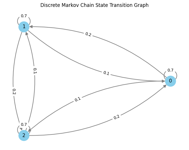
Step 1: For every of the $N(N-1)$ attainable transitions $i rightarrow j$ between $N$ states, draw an impartial level processes with parameter $p_{i,j}$. We now have an inventory of of occasion occasions for every transition. These will be visualised for a three-state Markov Chain as follows:
For every transition i->j, we draw transition occasions from some extent course of with parameter equivalent to the transition likelihood
This plot has one line for every transition from a state $i$ to a different state $j$. For every of those we drew transition factors from some extent course of. Discover how among the strains are denser – it’s because the corresponding transition possibilities are increased. That is the transition matrix I used:
To show this set of level processes right into a Markov chain, we have now to repeat the next steps ranging from time 0.
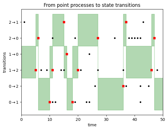
Assume at time $t$ the Markov chain is in state $i$. We contemplate the purpose processes for all transitions out of state $i$, and take a look at the earliest occasion in any of those sequences that occur after time $t$. Suppose this earlier occasion is at time $s+t$ and occurs within the level course of we drew for transition $i rightarrow j$. Our course of will then keep in state $i$ till time $s+t$, then we leap to to state $j$ and repeat the method.
That is illustrated within the following determine:
We begin the Markov chain in state $1$. We due to this fact give attention to the transitions $1rightarrow 0$ and $1 rightarrow 2$, as highlighted by the inexperienced space on the left aspect of this determine. We keep in state $1$ till we encounter a transition occasion (black dot) for both of those two transitions. This occurs after about 5 timesteps, as illustrated by the purple cross. At this level, we transition to state $2$, for the reason that first transition occasion was noticed within the $1 rightarrow 2$ row. Now we give attention to transition occasions for strains $2rightarrow 1$ and $2rightarrow 0$, i.e. the highest two rows. We do not have to attend too lengthy till a transition occasion is noticed, triggering a state replace to state $0$, and so forth. You’ll be able to learn off the Markov chain states from the place the inexperienced focus space lies.
This reparametrisation of a CTMC when it comes to underlying Poisson level processes now opens the door for us to simulate non-homogeneous CTMCs as properly. However, as this put up is already fairly lengthy, I am not going to let you know right here the right way to do it. Let that be your homework to consider: Return to course of 2 and course of 3 of simulating the homogeneous Poisson course of. Take into consideration what makes them homogeneous (i.e. the identical over time)? Which parts would change if the speed matrix wasn’t fixed over time? Which illustration can deal with non-constant charges extra simply?
Abstract
On this put up I tried to convey some essential, and I believe cool, instinct about steady time Markov chains. I focussed on exploring completely different representations of a Markov chain, every of which recommend a distinct method of simulating or sampling from the identical course of. Here’s a recap of some key concepts mentioned:
You’ll be able to reparametrise a homogeneous discrete Markov chain when it comes to ready occasions sampled from a geometrical distribution, and transition possibilities.
The geometric distribution has a memory-less property which has a deep reference to the Markov property of Markov chains.
One option to go steady is to contemplate a steady ready time distribution which preserves the memorylessness: the exponential distribution. This gave us our first illustration of a continuous-time chain, however it’s tough to increase this to non-homogeneous case the place the speed matrix might change over time.
We then mentioned completely different representations of discrete level processes, and famous (though didn’t show) their equivalence.
We may contemplate steady variations of those level processes, by changing discrete distributions by steady ones, once more preserving essential options comparable to memorylessness.
We additionally mentioned how a Markov chain will be described when it comes to underlying level processes: every state pair has an related level course of, and transitions occur when some extent course of related to the present state “fires”.
This was a redundant illustration of the Markov chain, inasmuch as most factors sampled from the underlying level processes didn’t contribute to the state evolution in any respect (within the final figures, most black dots lie exterior the inexperienced space, so you possibly can transfer their areas with out effecting the states of the chain).
Buildings will study and adapt. Suppose adaptive lighting that responds to temper. Occupancy sensors that predict demand—busy days, quiet moments. This enhances wellbeing and saves power: fewer over-lit, over-cooled workplaces that no one wants.
2. Command-Heart Dashboards for Property Managers
One display screen. All of your buildings. Stay information. Emptiness traits. Vitality spikes. Lease churn threat. Air high quality points. Predictive insights. You act—not react. Decisions turn out to be fast, knowledgeable, and well timed.
3. Augmented Actuality (AR) Meets Upkeep
No extra looking manuals or ready for specialists. With AR glasses, technicians get on the spot diagnostics layered over the very pipes or panels they’re fixing. Fixes occur quicker, safer, smarter.
4. Autonomous Constructing Operations
Constructing methods will self-heal. HVAC that recalibrates itself. Elevators that reroute foot visitors to keep away from congestion. Upkeep drones that examine façades. Buildings performing like well-oiled machines—not ready for you.
5. Sustainability Engineered In
From photo voltaic skins to green-roof sensors, buildings will steadiness power provide and demand in actual time. Renewable power goes from non-obligatory to integral. Carbon targets tracked dwell, reported mechanically. ESG turns into seamless—and measurable.
6. Sensible Neighborhoods, Not Simply Buildings
How is IoT utilized in actual property? Buildings will discuss to one another. Your workplace can hyperlink up parking, transport, retail, and shared areas—so all the things works in step. Information flows throughout clusters—enabling collaborative power sharing, crowd administration, and neighborhood-wide resilience.
Why this future just isn’t years away—and why you might want to act now:
Tech readiness: IoT in actual property, 5G and edge compute are already mature—and shrinking in value.
Tenant expectation: Well being, comfort, sustainability? They’re shifting from “wow options” to plain expectations.
Aggressive momentum: First movers are already rolling out complete good campuses, pulling forward of the curve. Linked applied sciences are on that threshold, and so they’re about to go from premium to baseline. For leaders, which means one factor: don’t wait to future-proof. Form the long run. Make your properties not simply locations, however predictors, protectors, and revenue facilities.
How Can Fingent Assist You Leverage Sensible Actual Property Administration
By partnering withFingent, you’re not simply shopping for software program — you’re constructing a future-ready ecosystem. We assist actual property companies combine PropTech options which might be scalable, safe, and tailor-made to your portfolio’s distinctive
One-size-fits-all? Not in actual property. Managing residential towers? Business hubs? Industrial parks the scale of small cities? Every comes with a unique rulebook—and a contemporary set of issues.
That’s why Fingent builds tailor-made good actual property administration options—ERP, lease monitoring, property valuation, HOA instruments—engineered to match the way you already run your online business. As a result of the very best tech doesn’t drive change. It suits proper in.
2. Sensible House Automation Built-in Seamlessly
We weave in good intercoms, keyless entry, good lighting—real-world comfort that enhances tenant security, satisfaction, and stickiness. Think about tenants unlocking with a faucet, doorways that greet them, and lights that know while you’re house. Right here’s an in depth story of how Fingent helped a distinguished consumer leverage good house automation for enhanced buyer expertise.
3. Tenant Engagement & Communications That Work
Sick of ready for solutions, repeating your self, and watching offers slip by the cracks? Fingent builds portals that consolidate tenant leads, help, and billing—automated and scalable. It’s like having a digital concierge that by no means sleeps and by no means drops the ball.
4. Legacy Programs Reworked, Not Tossed
Most corporations can’t afford to tear and exchange. Fingent bridges your legacy methods with future-ready tech—delivering transformation with out downtime, disruption, or drama. As much as 58% of actual property corporations wrestle right here—however options exist. Consequence: you modernize, strategize, and scale—with out the chaos.
5. ROI That Speaks Outcomes
Like for Rentmoji, our all-in-one answer supercharged operational scale. The consumer grew from simply 2 to 160 employees in two years. That’s effectivity in movement. We don’t simply ship tech. We ship scaling, progress, and ROI.
Sensible know-how in revolutionizing actual property. Realtors and property managers should act now to embrace the change and stay aggressive. Join with our proptech specialists right this moment and uncover what the new-age applied sciences have in retailer for you. Contact us now!
Information has turn into a neater commodity to retailer within the present digital period. With the benefit of getting plentiful information for enterprise, analyzing information to assist firms acquire perception has turn into extra important than ever.
In most companies, information is saved inside a structured database, and SQL is used to accumulate it. With SQL, we will question information within the type we wish, so long as the script is legitimate.
The issue is that, generally, the question to accumulate the information we wish is advanced and never dynamic. On this case, we will use SQL saved procedures to streamline tedious scripts into easy callables.
This text discusses creating information analytics automation scripts with SQL saved procedures.
Curious? Right here’s how.
# SQL Saved Procedures
SQL saved procedures are a group of SQL queries saved straight throughout the database. If you’re adept in Python, you’ll be able to consider them as features: they encapsulate a sequence of operations right into a single executable unit that we will name anytime. It’s useful as a result of we will make it dynamic.
That’s why it’s useful to grasp SQL saved procedures, which allow us to simplify code and automate repetitive duties.
Let’s strive it out with an instance. On this tutorial, I’ll use MySQL for the database and inventory information from Kaggle for the desk instance. Arrange MySQL Workbench in your native machine and create a schema the place we will retailer the desk. In my instance, I created a database known as finance_db with a desk known as stock_data.
We are able to question the information utilizing one thing like the next.
USE finance_db;

SELECT * FROM stock_data;
Basically, a saved process has the next construction.
As you’ll be able to see, the saved process can obtain parameters which can be handed into our question.
Let’s study an precise implementation. For instance, we will create a saved process to mixture inventory metrics for a selected date vary.
USE finance_db;
DELIMITER $$
CREATE PROCEDURE AggregateStockMetrics(
    IN p_StartDate DATE,
    IN p_EndDate DATE
)
BEGIN
    SELECT
        COUNT(*) AS TradingDays,
        AVG(Shut) AS AvgClose,
        MIN(Low) AS MinLow,
        MAX(Excessive) AS MaxHigh,
        SUM(Quantity) AS TotalVolume
    FROM stock_data
    WHERE
        (p_StartDate IS NULL OR Date >= p_StartDate)
      AND (p_EndDate IS NULL OR Date <= p_EndDate);
END $$
DELIMITER ;
Within the question above, we created the saved process named AggregateStockMetrics. This process accepts a begin date and finish date as parameters. The parameters are then used as circumstances to filter the information.
The process will execute with the parameters we cross. Because the saved process is saved within the database, you should utilize it from any script that connects to the database containing the process.
With saved procedures, we will simply reuse logic in different environments. For instance, I’ll name the process from Python utilizing the MySQL connector.
To do this, first set up the library:
pip set up mysql-connector-python
Then, create a perform that connects to the database, calls the saved process, retrieves the end result, and closes the connection.
That’s all it’s worthwhile to learn about SQL saved procedures. You may lengthen this additional for automation utilizing a scheduler in your pipeline.
# Wrapping Up
SQL saved procedures present a technique to encapsulate advanced queries into dynamic, single-unit features that may be reused for repetitive information analytics duties. The procedures are saved throughout the database and are simple to make use of from completely different scripts or purposes similar to Python.
I hope this has helped!
Cornellius Yudha Wijaya is a knowledge science assistant supervisor and information author. Whereas working full-time at Allianz Indonesia, he likes to share Python and information ideas through social media and writing media. Cornellius writes on quite a lot of AI and machine studying matters.
DirecTV’s Gemini streaming gadgets will quickly present you AI-generated advertisements that includes your face.
It’s partnering with Look, which can use your face to create AI avatars that includes shoppable merchandise, just like Google’s try-on purchasing function.
Look additionally powers lockscreen advertisements on telephones from main manufacturers.
The easiest way for many TV producers to extract worth from shoppers is to show advertisements. So why not take it up a notch with personalised focusing on? Or take it a step additional by exhibiting your digital clones on-screen to promote appropriate merchandise? That’s precisely what the US-based streaming {hardware} and repair supplier DirecTV goals to do with its newest growth.
The streaming big says the options are coming to its Gemini (to not be confused with Google’s Gemini AI) vary of gadgets in 2026. The so-called “AI-powered content material and commerce screensavers” are powered by Look, the identical platform that powers lock display advertisements on practically each main Android cellphone model, whereas labelling them as “wallpaper providers.” Look’s screensaver advertisements exist already on different Android-based streaming gadgets, together with ones supplied by Airtel in India, the place it’s already utilizing AI to generate a part of these screensaver advertisements.
Don’t wish to miss one of the best from Android Authority?
In DirecTV’s case, Look will present you photographs of sure merchandise, together with a QR code you’ll be able to scan along with your cellphone to add them, The Verge stories. Additionally, you will have the choice to insert a number of pictures to create a 30-second AI-generated spotlight video. Nevertheless, in contrast to Google, which creates digital avatars from precise merchandise, Look will solely present AI-generated merchandise which are related. In the event you like a glance, it should carry out a reverse search to match precise merchandise in its database, prompting you to finish the transaction in your cellphone.
As well as, Gemini streaming {hardware} may even show interactive advertisements from totally different classes, together with auto, native occasions and traits, well being, way of life, and journey, based mostly in your pursuits — presumably utilizing your watch historical past.
The DirecTV interface for large screens will not be the one platform to function personalised AI-generated advertisements. Earlier this yr, Look partnered with Samsung to show AI-generated variations of you dressed up in numerous outfits in your cellphone’s lock display. Thankfully, at the very least in Samsung’s case, these can be found solely on an opt-in (not opt-out) foundation.
It’s unclear the place it stands with DirecTV, however Look has already hinted at its plans to increase it to different surfaces, together with the launcher.
Thanks for being a part of our neighborhood. Learn our Remark Coverage earlier than posting.