All Courses - Page 254 of 276

Introduction to KV Cache Optimization Utilizing Grouped Question Consideration

Machine Learning

-

October 17, 2025

0

Introduction to KV Cache Optimization Utilizing Grouped Question Consideration

Residence

Desk of Contents

Introduction to KV Cache Optimization Utilizing Grouped Question Consideration
Understanding the KV Cache
Grouped Question Consideration
- What Is Grouped Question Consideration?
- How Grouped Question Consideration Reduces KV Cache?
Implementing KV Caching through Grouped Question Consideration
Abstract
- Quotation Info

Introduction to KV Cache Optimization Utilizing Grouped Question Consideration

Giant language fashions excel at processing in depth contexts, enabling them to generate coherent essays, perform multi-step reasoning, and preserve conversational threads over 1000’s of tokens. Nonetheless, as sequence lengths develop, so do the computational and reminiscence calls for throughout autoregressive decoding. Engineers should steadiness maximizing context window dimension and staying inside {hardware} limits.

On the coronary heart of this problem lies the key-value (KV) cache, which shops each previous key and worth tensor for every consideration head, thereby avoiding redundant computations. Whereas caching accelerates per-token technology, its reminiscence footprint scales linearly with the variety of consideration heads, sequence size, and mannequin depth. Left unchecked, KV cache necessities can balloon to tens of gigabytes, forcing trade-offs in batch dimension or context size.

Grouped Question Consideration (GQA) provides a center floor by reassigning a number of question heads to share a smaller set of KV heads. This easy but highly effective adjustment reduces KV cache dimension and not using a substantial impression on mannequin accuracy.

On this submit, we’ll discover the basics of KV cache, examine consideration variants, derive memory-savings math, stroll via code implementations, and share best-practice suggestions for tuning and deploying GQA-optimized fashions.

This lesson is the first of a 3-part sequence on LLM Inference Optimization — KV Cache:

Introduction to KV Cache Optimization Utilizing Grouped Question Consideration (this tutorial)
KV Cache Optimization through Multi-Head Latent Consideration
KV Cache Optimization through Tensor Product Consideration

To discover ways to optimize KV Cache utilizing Grouped Question Consideration, simply hold studying.

In search of the supply code to this submit?

Soar Proper To The Downloads Part

Understanding the KV Cache

Transformers compute, for every token in a sequence, three projections: queries $Q$ , keys $K$ , and values $V$ . Throughout autoregressive technology, at step $t$ , the mannequin should attend to all earlier tokens $1,dots,t-1$ .

With out caching, one would recompute

$K^{(ell)} = X^{(ell)} W_K,quad V^{(ell)} = X^{(ell)} W_V$

for each layer $ell$ and each previous token — an $O(t)$ value per token that rapidly turns into prohibitive.

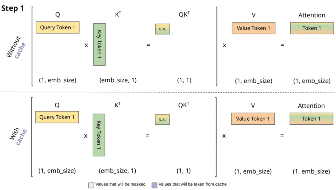
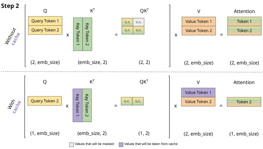
KV caching sidesteps this by storing the previous keys and values in reminiscence as they’re first computed, in order that at step $t$ , the mannequin solely must compute

$Q^{(ell)}_t = x_t W_Q$

after which carry out consideration towards the cached ${K^{(ell)}_{1:t-1},V^{(ell)}_{1:t-1}}$ (Figures 1 and a pair of).

As a result of every consideration head $h$ at layer $ell$ maintains its personal key and worth sequences of dimension $d_{text{head}}$ , the cache for that head and layer grows linearly within the context size $T$ .

**Determine 1:** No Distinction with and with out KV Cache for first token (supply: Chan, 2023).

Concretely, if there are $H$ consideration heads, and we retailer each keys and values in 2 bytes (FP16) per component, the per-layer KV cache dimension is

$text{Memory}_{text{layer}} = 2 times H times T times d_{text{head}} times 2 (text{bytes}).$

Over $L$ layers and a batch of dimension $B$ , the entire KV cache requirement turns into

$text{Memory}_{text{total}} = B times L times 2 times H times T times d_{text{head}} times 2.$

Past uncooked storage, every new token’s consideration computation should scan via the complete cached sequence, yielding a compute value proportional to

$text{FLOPs}_{text{per token}} propto H times d_{text{head}} times T.$

Thus, each reminiscence bandwidth (studying $K$ , $V$ ) and computation (dot-product of $Q$ towards all cached keys) scale linearly with the rising context.

KV caching dramatically reduces the work of recomputing ( $K$ ) and ( $V$ ), but it surely additionally makes the cache’s dimension and structure a first-class concern when pushing context home windows into the 1000’s of tokens.

**Determine 2:** From the second token onward, KV Caching makes use of already cached key and worth sequences for computing consideration scores (supply: Chan, 2023).

Grouped Question Consideration

What Is Grouped Question Consideration?

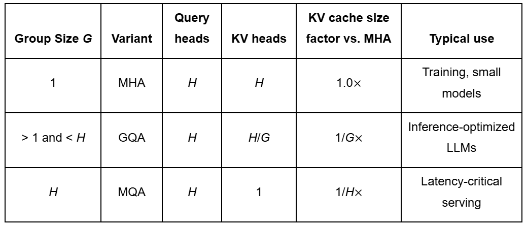
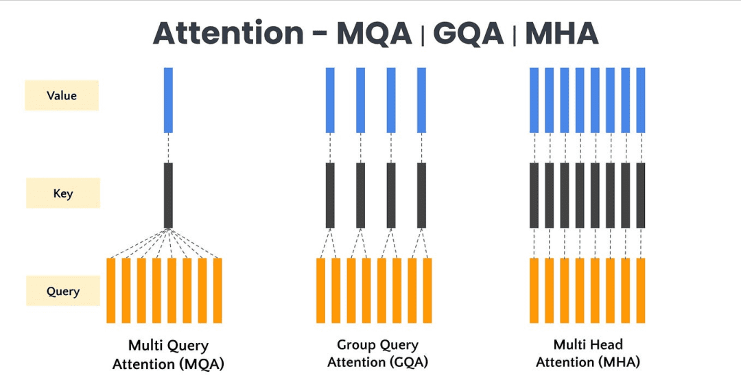
Grouped Question Consideration (GQA) modifies the usual multi-head consideration (MHA) by having a number of question heads share a lowered set of key and worth heads (Determine 3).

In vanilla MHA, the variety of key heads $H_{k}$ and worth heads $H_{v}$ equals the variety of question heads $H_{q}$ :

$H_{k} = H_{v} = H_{q}.$

GQA introduces a grouping issue $G$ in order that

$H_{kv} = displaystylefrac{H_{q}}{G},$

which means every group of $G$ question heads attends to a single shared key and worth head.

Regardless of this sharing, the question projections stay one per head:

$Q_i = X W_Q^{(i)},quad i=1,dots,H_q.$

Keys and values are computed solely per group: for group index $j=bigllfloor(i-1)/Gbigrrfloor+1$ , we now have

$K_j = X W_K^{(j)},quad V_j = X W_V^{(j)}.$

Throughout consideration, every question head $i$ makes use of the shared pair $(K_j, V_j)$ :

$text{Attn}(Q_i, K_j, V_j) =text{softmax} left(dfrac{Q_i K_j^top}{sqrt{d_{text{head}}}}right) V_j.$

By chopping the variety of key and worth projections from $H_q$ to $H_{kv}$ , GQA reduces each the parameter depend in $W_K$ and $W_V$ and the reminiscence wanted to retailer their outputs, whereas leaving the general mannequin dimension and ultimate output projection unchanged.

Primarily based on totally different values of $G$ , we are able to categorize consideration into the next sorts (Desk 1):

**Desk 1:** Comparability of consideration variants based mostly on group dimension G, KV cache utilization, and typical functions (supply: by the writer).

**Determine 3:** Comparability of Groped Question Consideration with Multihead Consideration and Multi-Question Consideration (supply: Shap, 2024).

How Grouped Question Consideration Reduces KV Cache?

The KV cache shops previous key and worth tensors of form $[Ttimes d_{text{head}}]$ for every head, the place $T$ is the present context size, and $b$ is the bytes per component (e.g., 2 for FP16).

In customary MHA, the per-layer cache reminiscence is

$text{Mem}_{text{MHA}} =2 times H_q times T times d_{text{head}} times b.$

Below GQA, solely $H_{kv}=H_q/G$ key and worth heads are saved, giving

$text{Mem}_{text{GQA}} =2 times H_{kv} times T times d_{text{head}} times b =displaystylefrac{2 times H_q times T times d_{text{head}} times b}{G}.$

Thus, the cache dimension shrinks by an element of ( $G$ ):

$displaystylefrac{text{Mem}_{text{GQA}}}{text{Mem}_{text{MHA}}} =displaystylefrac{1}{G}.$

Importantly, the compute value of the dot-product consideration — proportional to $H_q times d_{text{head}} times T$ — stays the identical.

This decouples reminiscence bandwidth from FLOPs, so decreasing the cache immediately interprets to quicker long-context inference with out altering per-token computational load.

Implementing KV Caching through Grouped Question Consideration

On this part, we’ll see how utilizing Grouped Question Consideration improves the inference time and KV Cache dimension. For simplicity, we’ll implement a toy transformer mannequin with 1 layer of a Grouped Question Consideration layer.

Grouped Question Consideration

We are going to begin by implementing the Grouped Question Consideration in PyTorch.

import torch
import torch.nn as nn
import time
import matplotlib.pyplot as plt

class GroupedQueryAttention(nn.Module):
    def __init__(self, hidden_dim, num_heads, group_size=1):
        tremendous().__init__()
        self.hidden_dim = hidden_dim
        self.num_heads = num_heads
        self.group_size = group_size
        self.kv_heads = num_heads // group_size
        self.head_dim = hidden_dim // num_heads

        self.q_proj = nn.Linear(hidden_dim, hidden_dim)
        self.k_proj = nn.Linear(hidden_dim, self.kv_heads * self.head_dim)
        self.v_proj = nn.Linear(hidden_dim, self.kv_heads * self.head_dim)
        self.out_proj = nn.Linear(hidden_dim, hidden_dim)

    def ahead(self, x, kv_cache):
        batch_size, seq_len, _ = x.dimension()

        # Venture queries, keys, values
        q = self.q_proj(x).view(batch_size, seq_len, self.num_heads, self.head_dim).transpose(1, 2)
        okay = self.k_proj(x).view(batch_size, seq_len, self.kv_heads, self.head_dim).transpose(1, 2)
        v = self.v_proj(x).view(batch_size, seq_len, self.kv_heads, self.head_dim).transpose(1, 2)

        # Append to cache
        kv_cache['k'] = torch.cat([kv_cache['k'], okay], dim=2)
        kv_cache['v'] = torch.cat([kv_cache['v'], v], dim=2)

        # Increase KV heads to match question heads
        k_exp = kv_cache['k'].repeat_interleave(self.group_size, dim=1)
        v_exp = kv_cache['v'].repeat_interleave(self.group_size, dim=1)

        # Scaled dot-product consideration
        scores = torch.matmul(q, k_exp.transpose(-2, -1)) / (self.head_dim ** 0.5)
        weights = torch.nn.practical.softmax(scores, dim=-1)
        attn_output = torch.matmul(weights, v_exp)

        # Merge heads
        attn_output = attn_output.transpose(1, 2).contiguous().view(batch_size, seq_len, self.hidden_dim)
        return self.out_proj(attn_output), kv_cache

We outline a grouped question consideration module on Traces 6-13. Right here, we inherit from nn.Module and seize the primary dimensions: hidden_dim, num_heads, and group_size. We compute kv_heads = num_heads // group_size to find out what number of key and worth heads we’ll truly challenge, and head_dim = hidden_dim // num_heads because the dimension per question head.

On Traces 15-18, we instantiate 4 linear layers: one every for projecting queries (q_proj), keys (k_proj), and values (v_proj), and a ultimate out_proj to recombine the attended outputs again into the mannequin’s hidden house.

On Traces 20-27, the ahead methodology begins by unpacking batch_size and seq_len from the enter tensor x. We then challenge x into queries, keys, and values. Queries are formed into (batch, num_heads, seq_len, head_dim) on Line 24, whereas keys and values use (batch, kv_heads, seq_len, head_dim) on Traces 25 and 26.

On Traces 29 and 30, we append these newly computed key and worth tensors alongside the time dimension into kv_cache, preserving all previous context for autoregressive decoding.

Subsequent, we align the cached key and worth heads to match the variety of question heads. On Traces 33 and 34, we use repeat_interleave to broaden every group’s cached ( $K$ , $V$ ) from kv_heads to num_heads so each question head can attend.

On Traces 37-39, we implement scaled dot-product consideration: we compute uncooked scores through q @ k_expᵀ divided by √head_dim, apply softmax to acquire consideration weights, after which multiply by v_exp to provide the attended outputs.

Lastly, on Traces 41-43, we merge the per‐head outputs again to (batch, seq_len, hidden_dim) and go them via out_proj, returning each the up to date consideration output and the expanded kv_cache.

Toy Transformer and Inference

Now that we now have carried out the grouped question consideration module, we’ll implement a 1-layer toy Transformer block that takes a sequence of enter tokens, together with KV Cache, and performs one feedforward go.

class TransformerBlock(nn.Module):
    def __init__(self, hidden_dim, num_heads, group_size=1):
        tremendous().__init__()
        self.attn = GroupedQueryAttention(hidden_dim, num_heads, group_size)
        self.norm1 = nn.LayerNorm(hidden_dim)
        self.ff = nn.Sequential(
            nn.Linear(hidden_dim, hidden_dim * 4),
            nn.ReLU(),
            nn.Linear(hidden_dim * 4, hidden_dim)
        )
        self.norm2 = nn.LayerNorm(hidden_dim)

    def ahead(self, x, kv_cache):
        attn_out, kv_cache = self.attn(x, kv_cache)
        x = self.norm1(x + attn_out)
        ff_out = self.ff(x)
        x = self.norm2(x + ff_out)
        return x, kv_cache

We outline a TransformerBlock class on Traces 1-11, the place the constructor wires collectively a grouped MultiHeadAttention layer (self.attn), two LayerNorms (self.norm1 and self.norm2), and a two-layer feed-forward community (self.ff) that expands the hidden dimension by 4× after which tasks it again.

On Traces 13-18, the ahead methodology takes enter x and the kv_cache, runs x via the eye module to get attn_out and an up to date cache, then applies a residual connection plus layer norm (x = norm1(x + attn_out)).

Subsequent, we feed this via the FFN, add one other residual connection, normalize once more (x = norm2(x + ff_out)), and at last return the reworked hidden states alongside the refreshed kv_cache.

The code under runs an inference to generate a sequence of tokens in an autoregressive method.

def run_inference(block, group_size=1):
    hidden_dim = block.attn.hidden_dim
    num_heads = block.attn.num_heads
    seq_lengths = checklist(vary(1, 101, 10))
    kv_cache_sizes = []
    inference_times = []

    kv_cache = {
        'okay': torch.empty(1, num_heads // group_size, 0, hidden_dim // num_heads),
        'v': torch.empty(1, num_heads // group_size, 0, hidden_dim // num_heads)
    }

    for seq_len in seq_lengths:
        x = torch.randn(1, 1, hidden_dim)  # One token at a time
        begin = time.time()
        _, kv_cache = block(x, kv_cache)
        finish = time.time()

        dimension = kv_cache['k'].numel() + kv_cache['v'].numel()
        kv_cache_sizes.append(dimension)
        inference_times.append(finish - begin)

    return seq_lengths, kv_cache_sizes, inference_times

On Traces 1-6, we outline run_inference, pull out hidden_dim and num_heads, and construct a listing of goal seq_lengths (1 to 101 in steps of 10), together with empty lists for kv_cache_sizes and inference_times.

On Traces 8-11, we initialize kv_cache with empty tensors for 'okay' and 'v' of form [1, num_heads//group_size, 0, head_dim] so it could possibly develop as we generate tokens.

Then, within the loop over every seq_len on Traces 13-17, we simulate feeding one random token x at a time into the transformer block, timing the ahead go, and updating kv_cache.

Lastly, on Traces 19-23, we measure the entire variety of components within the cached keys and values, append that to kv_cache_sizes, file the elapsed time to inference_times, after which return all three lists for plotting or evaluation.

Experiments and Evaluation

Lastly, we’ll check our implementation of grouped question consideration with totally different group sizes $G$ .

For every group dimension, we’ll plot the scale of the KV Cache and inference time as a perform of sequence size.

plt.determine(figsize=(12, 5))
plt.subplot(1, 2, 1)

for group_size in [1, 2, 4, 8, 16, 32]:
    gqa_block = TransformerBlock(hidden_dim=4096, num_heads=32, group_size=group_size)
    seq_lengths, sizes, instances = run_inference(gqa_block, group_size=group_size)
    plt.plot(seq_lengths, sizes, label="GQA : {}".format(group_size))

plt.xlabel("Generated Tokens")
plt.ylabel("KV Cache Dimension")
plt.title("KV Cache Progress")
plt.legend()

plt.subplot(1, 2, 2)
for group_size in [1, 2, 4, 8, 16, 32]:
    gqa_block = TransformerBlock(hidden_dim=4096, num_heads=32, group_size=group_size)
    seq_lengths, sizes, instances = run_inference(gqa_block, group_size=group_size)
    plt.plot(seq_lengths, instances, label="GQA : {}".format(group_size))


plt.xlabel("Generated Tokens")
plt.ylabel("Inference Time (s)")
plt.title("Inference Velocity")

plt.legend()

plt.tight_layout()
plt.present()

On Traces 1 and a pair of, we arrange a 12×5-inch determine and declare the primary subplot for KV cache development.

Between Traces 4-7, we loop over numerous group_size values, instantiate a TransformerBlock for every, name run_inference to assemble sequence lengths and cache sizes, and plot the KV cache dimension versus the variety of generated tokens.

On Traces 14-18, we change to the second subplot, repeat the loop to gather and plot inference instances towards token counts, and at last, on Traces 21-28, we set axis labels, add a title and legend, tighten the structure, and name plt.present() to render each charts (Determine 4).

**Determine 4:** Discount in KV cache dimension and inference time through the use of Group Question Consideration (supply: picture by the writer).

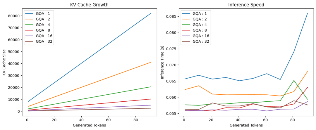
As proven in Determine 4, utilizing grouped question consideration considerably reduces the KV cache dimension and inference time in comparison with vanilla multihead self-attention (group dimension 1).

What’s subsequent? We suggest PyImageSearch College.

Course data:
86+ whole courses • 115+ hours hours of on-demand code walkthrough movies • Final up to date: October 2025
★★★★★ 4.84 (128 Scores) • 16,000+ College students Enrolled

I strongly imagine that when you had the fitting trainer you could possibly grasp pc imaginative and prescient and deep studying.

Do you suppose studying pc imaginative and prescient and deep studying needs to be time-consuming, overwhelming, and sophisticated? Or has to contain advanced arithmetic and equations? Or requires a level in pc science?

That’s not the case.

All you must grasp pc imaginative and prescient and deep studying is for somebody to elucidate issues to you in easy, intuitive phrases. And that’s precisely what I do. My mission is to alter training and the way advanced Synthetic Intelligence subjects are taught.

Should you’re critical about studying pc imaginative and prescient, your subsequent cease must be PyImageSearch College, probably the most complete pc imaginative and prescient, deep studying, and OpenCV course on-line immediately. Right here you’ll discover ways to efficiently and confidently apply pc imaginative and prescient to your work, analysis, and tasks. Be a part of me in pc imaginative and prescient mastery.

Inside PyImageSearch College you will discover:

&examine; 86+ programs on important pc imaginative and prescient, deep studying, and OpenCV subjects
&examine; 86 Certificates of Completion
&examine; 115+ hours hours of on-demand video
&examine; Model new programs launched repeatedly, guaranteeing you’ll be able to sustain with state-of-the-art strategies
&examine; Pre-configured Jupyter Notebooks in Google Colab
&examine; Run all code examples in your net browser — works on Home windows, macOS, and Linux (no dev surroundings configuration required!)
&examine; Entry to centralized code repos for all 540+ tutorials on PyImageSearch
&examine; Simple one-click downloads for code, datasets, pre-trained fashions, and so forth.
&examine; Entry on cell, laptop computer, desktop, and so forth.

Click on right here to hitch PyImageSearch College

Abstract

We start by framing the problem of lengthy‐context inference in transformer fashions. As sequence lengths develop, storing previous key and worth tensors within the KV cache turns into a significant reminiscence and bandwidth bottleneck. To deal with this, we introduce Grouped Question Consideration (GQA), an architectural modification that permits a number of question heads to share a smaller set of key-value heads, thereby decreasing the cache footprint with minimal impression on accuracy.

Subsequent, we unpack the mechanics of KV caching — why transformers retailer per‐head key and worth sequences, how cache dimension scales with head depend $H$ , context size $T$ , and mannequin depth $L$ , and the ensuing latency strain from studying giant caches every token. We then formally outline GQA, displaying how the grouping issue $G$ reduces the variety of KV projections from $H$ to $H/G$ and yields a $1/G$ discount in cache reminiscence. We illustrate this with equations and intuitive diagrams, contrasting vanilla multi‐head consideration, multi‐question consideration, and the GQA center floor.

Lastly, we stroll via a hands-on implementation: constructing a toy TransformerBlock in PyTorch that helps arbitrary GQA groupings, wiring up KV cache development, and operating inference experiments throughout group sizes. We plot how cache dimension and per-token inference time evolve for $G in {1,2,4,8,16,32}$ , analyze the memory-latency trade-off, and distill sensible tips for selecting $G$ and integrating GQA into real-world LLM deployments.

Quotation Info

Mangla, P. “Introduction to KV Cache Optimization Utilizing Grouped Question Consideration,” PyImageSearch, P. Chugh, S. Huot, A. Sharma, and P. Thakur, eds., 2025, https://pyimg.co/b241m

@incollection{Mangla_2025_intro-to-kv-cache-optimization-using-grouped-query-attention,
  writer = {Puneet Mangla},
  title = {{Introduction to KV Cache Optimization Utilizing Grouped Question Consideration}},
  booktitle = {PyImageSearch},
  editor = {Puneet Chugh and Susan Huot and Aditya Sharma and Piyush Thakur},
  12 months = {2025},
  url = {https://pyimg.co/b241m},
}

To obtain the supply code to this submit (and be notified when future tutorials are printed right here on PyImageSearch), merely enter your e mail tackle within the type under!

Obtain the Supply Code and FREE 17-page Useful resource Information

Enter your e mail tackle under to get a .zip of the code and a FREE 17-page Useful resource Information on Laptop Imaginative and prescient, OpenCV, and Deep Studying. Inside you will discover my hand-picked tutorials, books, programs, and libraries that can assist you grasp CV and DL!

The submit Introduction to KV Cache Optimization Utilizing Grouped Question Consideration appeared first on PyImageSearch.

Who’s in Cost of Your AI Technique? SAS CIO Explains Why It Issues

IT

Dr. Mike

-

October 17, 2025

0

Who’s in Cost of Your AI Technique? SAS CIO Explains Why It Issues

Among the many prime gadgets holding CIOs up at evening is knowing who ought to lead the AI technique at their organizations.

SAS CIO Jay Upchurch instructed InformationWeek that CIOs world wide are grappling with figuring out the place the duty lies for organizational AI methods and who ought to take the lead on company-wide AI mandates. The CIO will, after all, implement AI applied sciences, Upchurch defined, however selecting who leads the cost on AI technique is a separate problem.

“Is it pushed from the highest down, as a board or CEO mandate? Is it a groundswell of curiosity from staff?” Upchurch mentioned.

SAS, for its half, has taken a multi-pronged strategy to implementing its AI technique throughout the group, guaranteeing buy-in from each the chief group and the worker base.

Having help from management throughout the group has been important to realizing this broad-based strategy to AI implementation. Every division throughout the group has a tech chief who can advocate for his or her division and assist the IT group higher perceive their expertise necessities, Upchurch mentioned.

At a latest SAS occasion, CTO Bryan Harris additionally emphasised the significance of company-wide buy-in for AI when deploying the expertise. Step one in AI deployments, he mentioned, is “constructing belief between you and your workforce.”

Associated:InformationWeek Podcast: Below AI, Is the Citizen Developer Period Over?

(Supply: Shane Snider/Knowledge Heart Information) Bryan Harris, CTO of SAS, mentioned the corporate’s strategy to AI at a SAS Championship 2025 occasion.

“Firms want daring and inspirational leaders who spend money on their workforce by way of this continued change,” Harris mentioned. “As you spend money on individuals and their abilities, you construct belief. And constructing belief will increase AI adoption, which in flip will increase your aggressive benefit. It is all related.”

Among the many leaders in control of AI technique at SAS is an AI working council that features eight individuals from the chief group and different ranges of administration. The council meets frequently to “evaluate requests for brand new AI which may come into the enterprise,” Upchurch mentioned.

One subject the council has mentioned is how regional laws may have an effect on the deployment of recent AI applied sciences within the varied international locations the place SAS does enterprise.

“So it is not IT or authorized saying ‘sure or no.’ It is a group of people which have an curiosity within the security and safety of our staff, our knowledge, our firm’s knowledge, and our clients’ knowledge,” Upchurch mentioned.

A Productiveness-First Strategy to AI

With out enterprise-wide help, IT groups run the danger of rolling out an costly AI that sits on a shelf amassing mud, he added. That is partly why SAS selected to first roll out AI to help worker productiveness.

Associated:How a CIO Can Wake Up a Slumping IT Group

Instruments that automate and help with mundane duties, like Microsoft Copilot or Anthropic’s Claude, could be tailor-made to staff’ particular roles, serving to them really feel valued and giving them the “present of time” to give attention to higher-impact work, Upchurch mentioned.

Harris mentioned the AI give attention to productiveness has already proved a boon for the corporate. “When [employees] offload this tedious work, they’ve extra time to assume, consider and make higher choices,” he mentioned. “Nobody is debating the ROI of this primary section.”

Advantages of an AI-Prepared Workforce

Certainly, SAS staff are pretty educated about AI and have been fast to use it, Upchurch mentioned. In September, SAS carried out a Microsoft Copilot license for SAS staff to construct their very own AI brokers to help their productiveness targets. By early October, staff had created 760 AI brokers.

Having an AI-literate worker base has been useful “when it comes to velocity and effectivity” for deploying AI throughout the group, Upchurch added.

SAS’ 12,000 staff are “extremely knowledgeable about what AI is and learn how to do it the best approach,” Upchurch mentioned. “After I’ve talked to numerous my CIO friends, they battle with that, in order that they’re out chasing knowledge literacy or AI literacy or one thing else with their very own worker base.”

Associated:Human-AI Collaboration Is the New Teamwork. Are We Prepared?

Nonetheless, change administration is just not a straightforward process for any group, Upchurch mentioned.

“You possibly can clear knowledge up, and with sufficient time and money you are able to do a venture and ship a functionality, however getting individuals to embrace and alter their mindset is tough work,” he mentioned. “The best expertise, the best tasks, can land flat if the corporate or the group is just not able to obtain it, and that is very true in AI.”

What’s Subsequent for SAS’ AI Technique: Reimagining Workflows

After worker productiveness — the primary space of focus within the firm’s inside AI technique — SAS will give attention to infusing AI into work processes to “reimagine workflows,” and utilizing AI for autonomous operations, Upchurch mentioned. The intention is to rethink how work will get executed with AI, as a substitute of merely automating present processes.

In the long run, Upchurch mentioned SAS is concentrated on utilizing AI for autonomous operations resembling computerized software program anomaly detection and remediation. In the meantime, it is the “superb innovation and curiosity tradition,” not the expertise, that accounts for the corporate’s progress.

“After we see these two issues come collectively, it fuels each other, and it simply continues to breed success for us,” he mentioned.

8 Excessive-Demand AI Jobs in 2025

Artificial Intelligence

Dr. Mike

-

October 17, 2025

0

Are you involved concerning the affect of AI in your career? You’re not alone.

With Synthetic Intelligence altering the world, and nonetheless altering it at a staggering tempo, folks all all over the world are asking themselves how they are often related -or even ahead- of the occasions of clever automation.

Organizations are making use of AI to automate processes, optimize decision-making, and supply a better buyer expertise. This wave of adoption has generated an enormous demand for skilled personnel with the potential to slender the hole between AI applied sciences and precise enterprise necessities.

On this article, we’ll talk about the 8 high-demand AI jobs in 2025 and what they entail, the abilities required to work, and how one can put together to work in these positions. These positions not solely have excessive progress prospects and aggressive pay but additionally the chance to safe probably the most profitable careers in 2025 and past.

Why AI Careers Are Booming in 2025

With the adoption of AI expertise in enterprise processes has led to a 25% productiveness increase within the manufacturing enterprise, by which over 35 p.c of e-commerce revenues come by AI-based methods. The AI job market represents a big selection of future-proof employment alternatives to those that are keen to be part of AI-powered job roles that deliver the following wave of automation & data-driven decision-making throughout industries.

8 Excessive-Demand AI Jobs in 2025

1. AI Engineer

The AI Engineers are essential contributors to the event of AI as they’re engaged of their actions, which embody creating AI options & growing their purposes in real-world problem-solving wants.

The on a regular basis duties of AI Engineers encompass mannequin growth exercise & enterprise management involvement.
They align AI options & integrative exercise amongst AI instruments, merchandise, & providers, incomes an annual median wage of $145,080

To develop into profitable within the space, one must grasp Python programming, possess the information of such frameworks as TensorFlow or PyTorch, & know discover the answer to difficult issues.

Moreover, should you’re simply beginning with Synthetic Intelligence, Grasp Synthetic Intelligence by Nice Studying is right to discover the basics of AI, machine studying, deep neural networks, GenAI, & to construct key expertise within the newest applied sciences.

2. Machine Studying Engineer

A Machine Studying Engineer develops computerized studying algorithms that may allow computer systems to be taught by the datasets & mechanically enhance their efficiency in a minimal quantity of human code.

Machine studying engineers perform their roles by creating, testing, & implementing machine studying fashions & automating actions.
The common annual wage of a machine studying engineer within the US is $109,143.
Their position is essential as a result of they design and implement clever methods, resembling advice engines and fraud detection fashions, that assist organizations make smarter choices, optimize operations, and ship customized person experiences.

These trying to construct experience on this area typically pursue specialised applications, resembling an on-line MS in Synthetic Intelligence and Machine Studying, which give a complete basis in programming, statistics, and operations of ML frameworks.

3. Information Scientist

Information Scientists research in depth databases to generate sensible info that guides enterprise planning. The position of Information Scientists stays important all through the e-commerce, finance, and healthcare sectors, as they make the most of knowledge insights to boost operational effectivity and sample prediction.

The scope of their duties consists of growing knowledge fashions, performing predictive analytics, and supporting key firm choices.
Skilled success for knowledge analysts requires experience in each knowledge evaluation strategies and programming expertise, in addition to machine studying practices and statistical strategies.

To attain success within the discipline, you will need to choose an appropriate instructional path. Formal levels, together with Bachelor’s and Grasp’s applications, set up the essential theoretical and sensible foundations, whereas specialised choices, such because the MS in Information Science program, additional sharpen the skilled expertise that companies urgently want and permit you to earn the common annual wage of $65,674.

Carefully associated to knowledge science roles, Information Architects play a significant half in designing the infrastructure that helps large-scale analytics and AI methods. Be taught extra about what a Information Architect does, required expertise, and profession pathways on this information: Find out how to develop into a Information Architect.

4. AI Analysis Scientist

AI Analysis Scientists advance AI expertise by growing novel algorithms and conducting analysis experiments that propel the sector ahead.

The analysis staff conducts deliberate experiments and publishes their outcomes by collaboration with tutorial establishments and industrial companions.
To excel on this place, one requires professional-level mathematical expertise, mixed with in depth studying expertise and a stable understanding of analysis strategies.
AI Analysis Scientists are essential in growing technological advances, which decide how AI purposes evolve all through time.

Understanding the key duties and instruments of a Information Analyst may assist construct a powerful base for progress in AI-focused roles, as many professionals start their careers as Information Analysts earlier than advancing into knowledge science or AI specializations, incomes a median annual wage of $115,443 as an AI analysis scientist within the US.

5. Robotics Engineer

Throughout the discipline of robotics engineering, professionals design and develop clever robotic methods to automate varied industrial operations, starting from manufacturing actions to logistics and healthcare purposes, and earn an common annual wage of $120,997 per 12 months.

The duties of those professionals embody robotic creation, coding actions, check runs, and system upkeep.
They develop clever machines by an ideal mix of robotics engineering and Synthetic Intelligence integration capabilities to execute autonomous advanced duties.
The implementation of automation by industries drives continuous growth within the want for Robotics Engineers and exhibits no signal of slowing down.

Automation additionally extends past robotics into software program high quality and efficiency testing. Professionals aiming to make sure the reliability of AI methods can discover a profession as an Automation Check Engineer, answerable for designing check frameworks and enhancing AI mannequin effectivity. Be taught extra on this detailed Automation Check Engineer Profession Information.

6. Pc Imaginative and prescient Engineer

Via the event of methods, Pc Imaginative and prescient Engineers allow computer systems to grasp visible info from photos and video content material.

Their programming empowers purposes to acknowledge faces, drive autonomous autos, and ship augmented actuality capabilities.
Incomes the common annual wage of $168,803, these specialists are answerable for creating and fine-tuning algorithms that allow machines to interpret visible knowledge, thereby bridging the hole between uncooked pictures and actionable insights for real-world purposes, resembling medical diagnostics and robotics.
The required skills for this discipline embody deep studying strategies, picture processing, and superior laptop imaginative and prescient strategies, expertise which might be more and more valued as knowledge turns into central for enterprise options and innovation.

7. AI Chatbot Developer / NLP Engineer

The mixture of AI Chatbot Builders and NLP Engineers is reworking how companies work together with clients by growing methods and conversational brokers that may perceive and generate human language.

These professionals design multi-tiered chatbots and construct refined NLP fashions to strengthen dialogue and person engagement. They collaborate intently with different engineers to create methods that may comprehend human voice and textual content and react accordingly, with the common annual wage of an NLP engineer $86,193.
Their work requires competency in NLP, Python, and mastery of chatbot frameworks, in addition to an understanding of combine AI fashions for responsive, context-aware conversations.
A powerful basis, resembling one constructed by a complete Pure Language Processing tutorial, is essential for excelling on this discipline.

As LLM and NLP AI fashions proceed to be into demand with AI chatbot developer, a associated and fast-emerging position is that of the Immediate Engineer who designs and optimizes the inputs that information AI fashions to supply related outputsis additionally on the increase.

You possibly can discover extra about develop into a immediate engineer and construct the precise ability set for this GenAI-driven position.

8. AI Product Supervisor

The position of the AI Product Supervisor exists to merge technical operations with enterprise priorities, making certain that AI venture effectivity aligns with organizational ideas. For an in depth understanding of what the position entails, discover this complete information on AI Product Supervisor expertise, duties, and profession progress.

Incomes the common annual wage of $128,091, these professionals steer product path and oversee growth duties, sustaining efficient staff relationships all through the method.
Data of product administration, AI proficiency, communication expertise, and enterprise understanding are important competencies.
The central significance of AI Product Managers in enterprise technique growth is rising, as they’re essential for attaining profitable AI implementation and maximizing the worth of AI investments.

CONCLUSION

Within the 12 months 2025, AI may have quite a few alternatives with many rewarding roles that shall be supplied to people with applicable competencies.

Amongst these professions, AI Engineers, Information Scientists, NLP consultants, and AI Product managers are the careers that enhance the technological and enterprise functioning of recent society.Those that wish to develop into leaders within the space of educational innovation and superior expertise analysis can apply to get a Doctorate in AI and Machine Studying to discover new technological frontiers.

On Unbiased MCMC with couplings – Robin Ryder’s weblog

Statistics

Dr. Mike

-

October 17, 2025

0

On Unbiased MCMC with couplings – Robin Ryder’s weblog

Pierre Jacob, John O’Leary and Yves Atchadé’s wonderful paper on Unbiased MCMC with couplings will likely be learn on the Royal Statistical Society tomorrow; Pierre has already introduced the paper on the Statisfaction weblog.
Though we received’t be current tomorrow, we’ve got learn it at size in our native studying group with Xian Robert and PhD college students Grégoire Clarté, Adrien Hairault and Caroline Lawless, and have submitted the next dialogue.

We congratulate the authors for this wonderful paper.

In “conventional” MCMC, it’s customary to verify that stationarity has been attained by operating a small variety of parallel chains, initiated at completely different beginning factors, to confirm that the ultimate distribution is unbiased of the initialization — although the one versus a number of chain(s) debate errupted from the beginning with Gelman and Rubin (1992) versus Geyer (1992).

As famous by the authors, a nasty selection of the preliminary distribution can result in poor properties. In essence, this happens and stays undetected for the present proposal as a result of the coupling of the chains happens lengthy earlier than the chain reaches stationarity. We wish to make two ideas to alleviate this situation, and therefore add a stationarity verify as a byproduct of the run.

The chains $X$ and $Y$ have to have the identical preliminary distribution, however completely different pairs of chains on completely different parallel cores can afford completely different preliminary distributions. The ensuing estimator stays unbiased. We’d subsequently recommend that parallel chains be initiated from distributions which put weight on completely different elements of the parameter area. Concepts from the Quasi-Monte Carlo literature (see Gerber & Chopin 2015) may very well be used right here.
We additionally word that though the marginal distributions of $X$ and $Y$ have to be similar, any joint distribution on $(X,Y)$ produces an unbiased algorithm. We’d recommend that it’s preferable that $X$ and $Y$ meet (shortly) after the chains have reached stationarity. Right here is one attainable technique to this finish: let $p$ and $p'$ be two distributions which put weight on completely different elements of the area, and $Zsim Bernoulli(1/2)$ . If $Z=0$ , take $X_0sim p$ and $Y_0sim p'$ , else take $X_0sim p'$ and $Y_0sim p$ . The marginal distribution of each $X_0$ and $Y_0$ is $frac12(p+p')$ , however the two chains will begin in several elements of the parameter area and are more likely to meet after they’ve each reached stationarity.

The best algorithm is one which provides an accurate reply when it has converged, and a warning or error when it hasn’t. MCMC chains which haven’t but reached stationarity (for instance as a result of they haven’t discovered all modes of a multimodal distribution) might be arduous to detect. Right here, this situation is extra more likely to be detected since it will result in the coupling not occuring: $mathbb E[tau]$ is giant, and it is a function, because it warns the practitioner that their kernel is ill-fitted to the goal density.

Revealed by Robin Ryder

View all posts by Robin Ryder

Revealed
10/12/2019

The Orionid meteor bathe peaks below darkish, moonless skies subsequent week. This is the best way to see it

Science

Dr. Mike

-

October 17, 2025

0

The Orionid meteor bathe peaks below darkish, moonless skies subsequent week. This is the best way to see it

In the event you occur to glimpse a “taking pictures star” earlier than daybreak throughout the subsequent a number of days, there is a good probability that what you noticed was a fraction left behind in area by the well-known Halley’s Comet. For it’s throughout the third week of October {that a} meteor show spawned by the particles shed by Halley reaches its peak: the Orionid meteor bathe.

The Orionids aren’t one of many 12 months’s richest meteor shows. If the August Perseids and December Geminids might be thought-about the “first string” among the many annual meteor showers by way of brightness and reliability, then the Orionids are on the junior varsity crew.

And this will probably be a superb 12 months to search for them, because the moon will arrive at new part on Tuesday morning, Oct. 21 at the exact same time that the Orionids are reaching their most and therefore won’t pose any hindrance in any respect for these waiting for these fiery streaks throughout their prime predawn viewing hours. Good!

The meteor moniker “Orionid” comes from the truth that the radiant — that spot on the sky from the place the meteors seem to fan out from — is simply above Orion‘s second brightest star, ruddy Betelgeuse.

Orion, in fact, is a winter constellation. At this second, in early autumn, he seems forward of us in our path across the solar, and as such has not fully risen above the japanese horizon till after 11:00 p.m. native daylight time. A number of hours later, between 4 and 5:00 a.m. — Orion will probably be excessive within the sky towards the south-southeast. The upper within the sky Orion is, the extra meteors will seem everywhere in the sky. The Orionids are considered one of only a handful of recognized meteor showers that may be noticed equally effectively from each the Northern and Southern Hemispheres.

However to see the best variety of meteors, do not look within the path of the radiant, however relatively about 30 levels from it, within the path of the purpose instantly overhead (the zenith). Your clenched fist held at arm’s size is roughly equal to 10 levels, so trying “three fists” up from Betelgeuse will probably be the place to pay attention your view.

An evening sky map displaying the Orionids meteor bathe. (Picture credit score: Starry Evening/Chris Vaughan)

Halley’s legacy

As famous on the onset of this dialogue, the Orionids have an illustrious lineage: Just like the Eta Aquariid meteors of early Could, they’re bits of particles shed way back by Halley’s Comet. The 2 showers are basically one and the identical; Earth intersects a single, broad stream of meteoroids at two locations in its orbit on reverse sides of the solar. Usually, just like the Eta Aquarids, Orionid meteors are usually dim and never effectively seen from city areas, so it is instructed that you simply discover a darkish (and protected) rural location to see the perfect Orionid exercise.

“They’re simply recognized … from their pace,” write David Levy and Stephen Edberg in Observe: Meteors, an Astronomical League guide. “At 66 kilometers (41 miles) per second, they seem as quick streaks, quicker by a hair than their sisters, the Eta Aquarids of Could. And just like the Eta Aquarids, the brightest have a tendency to go away long-lasting trains. Fireballs are attainable three days after most.” This side is undoubtedly linked in a roundabout way to the make-up of Halley’s Comet.

A glowing light house stands on the edge of a coastline where above it a meteor streaks in the night sky

The Orionids are a delight for any skywatcher. (Picture credit score: Mountain Gentle Images Inc/Getty Pictures)

The bathe is definitely a fancy of a number of sub-showers with totally different maxima unfold over a number of days. Halley’s Comet’s final go to by means of the internal photo voltaic system was within the late winter of 1986 and it’s due again within the midsummer of 2061. However every time it has swept previous the solar — and it has carried out so in all probability numerous lots of, if not 1000’s of occasions — it has launched tiny particles, largely ranging in dimension from mud to sand grains, which journey close to and alongside the comet’s orbit, creating a unclean path of particles that has been distributed kind of uniformly all alongside its total orbit.

The comet bits have additionally unfold a good distance from it sideways, which is why among the particles now intersect the Earth despite the fact that the comet’s orbit doesn’t. Concerning the 12 months 530 A.D. Halley’s orbit intersected that of the Earth. Presently, the least distance between the 2 orbits is 6,042,000 miles (9,710,000 km).

Observing ideas

Orionid visibility extends from Oct. 16 to 26, with peak exercise of maybe 15 to 30 meteors per hour approaching the morning of Oct. 21. Step outdoors earlier than dawn on any of those mornings and for those who catch sight of a meteor, there’s a couple of 75 % probability that it possible is a by-product of Halley’s Comet. The final Orionid stragglers often seem someday in early to mid-November.

Remember to bundle up very warmly; maybe convey a sleeping bag. Discover a darkish spot with an open view of the sky. The much less mild air pollution, the higher; a bathe like this one which’s wealthy in faint meteors is very onerous hit by synthetic skyglow. The path to observe is wherever your sky is darkest. Lie again, let your eyes adapt to the evening, and be affected person.

Good luck and clear skies!

Joe Rao serves as an teacher and visitor lecturer at New York’s Hayden Planetarium. He writes about astronomy for Pure Historical past journal, Sky and Telescope and different publications.

Weekend Movies — Would-Be Tyrants and Actual-Life Giants

Epidemiology

Dr. Mike

-

October 17, 2025

0

Weekend Movies — Would-Be Tyrants and Actual-Life Giants

That is a unprecedented piece of tv. It’s, virtually with out fail, pitch good. It acknowledges the gravity of the second whereas conserving a wholesome sense of perspective. As he himself factors out, the destiny of a chat present is trivial in comparison with many different issues happening, however the points it raises are usually not trivial in any respect.

For these of us who’re approach too into the historical past of the medium, the monologue opens with a 65-year-old callback to maybe the primary discuss present censorship scandal.

As Josh Marshall and lots of others have identified, presumably the worst consequence for Sinclair is having its viewers be taught extra about who owns their native stations. A couple of years in the past, John Oliver did a wonderful section on Sinclair that has solely develop into extra related.

I notably appreciated the best way round 1:20 Oliver adopted up his teasing of native information by acknowledging that native tv journalists usually do extraordinary work, and have, to a point, stepped as much as fill the void left by the decline of newspapers.

Lastly, simply to finish on a much less infuriating word, here’s a very cool story concerning the making of The Princess Bride.

“The Princess Bride” turns 38 right now.

Right here’s an amazing story about Andre the Big — as advised by Mandy Patinkin.

[image or embed]

— Carl Quintanilla (@carlquintanilla.bsky.social) September 25, 2025 at 7:27 AM

Signal Restricted SVAR in GAUSS

Econometrics

Dr. Mike

-

October 17, 2025

0

by

Eric

· Printed

Might 20, 2025
· Up to date

June 18, 2025

Introduction

In structural vector autoregressive (SVAR) modeling, one of many core challenges is figuring out the structural shocks that drive the system’s dynamics.

Conventional identification approaches typically depend on short-run or long-run restrictions, which require robust theoretical assumptions about contemporaneous relationships or long-term conduct.

Signal restriction identification supplies better flexibility by permitting economists to specify solely the route, constructive, adverse, or impartial, of variable responses to shocks, based mostly on principle.

On this weblog, we’ll present you the best way to implement signal restriction identification utilizing the brand new GAUSS process, svarFit, launched in TSMT 4.0.

We’ll stroll via the best way to:

Specify signal restrictions.
Estimate the SVAR mannequin.
Interpret the ensuing impulse response features (IRFs).

By the top of this information, you’ll have a stable understanding of the best way to apply signal restrictions to uncover significant financial relationships.

What are Signal Restrictions?

Signal restrictions are a way of figuring out structural shocks in SVAR fashions by specifying the anticipated route of response of endogenous variables.

Signal restrictions:

Don’t impose actual constraints on parameter values or long-term impacts; they solely require that impulse responses transfer in a specific route for a specified interval.
Are versatile and fewer reliant on strict parametric assumptions than different identification strategies.
Depend on qualitative financial insights, making them much less liable to mannequin specification errors.

For instance, in a financial coverage shock, financial principle would possibly counsel that a rise in rates of interest ought to result in a decline in output and inflation within the brief run. An SVAR signal restriction identification method would implement these directional actions.

Estimating SVAR Fashions in GAUSS

The svarFit process, obtainable in TSMT 4.0, gives an all-in-one device for:

Estimating reduced-form parameters of VAR fashions.
Implementing structural identification.
Deriving impulse response features (IRFs), forecast error variance decompositions (FEVDs), and historic decompositions (HDs).

Whereas the process supplies intuitive defaults for fast and simple estimation, it additionally gives the pliability to completely customise your mannequin.

For an in depth, step-by-step walkthrough of the estimation course of, check with my earlier weblog put up:
Estimating SVAR Fashions with GAUSS.
That put up gives steering on organising the mannequin, estimating reduced-form parameters, and performing structural identification.

Implementing Signal Restrictions with `svarFit`

The svarFit process means that you can specify signal restrictions as a structural identification technique. That is accomplished in three major steps:

Set the identification technique to signal restrictions.
Outline the signal restriction matrix.
Specify the shock variables and impacted horizons.

Instance: Signal Restricted Responses to Provide, Demand, and Financial Coverage Shocks

Let’s discover an empirical instance capturing the dynamic relationships between inflation, unemployment, and the federal funds charge.

We’ll impose economically significant signal restrictions to determine three key shocks:

Shock Sort	Inflation	Unemployment	Federal Funds Charge
Provide Shock	–	–	–
Demand Shock	+	–	+
Financial Coverage Shock	–	+	+

These restrictions enable us to use financial principle to untangle the underlying structural drivers behind noticed actions within the knowledge.

Step One: Loading Our Knowledge

Step one in our mannequin is to load the information from the data_narsignrestrict.dta file.

/*
** Knowledge import
*/
fname = "data_narsignrestrict.dta";
data_shortrun = loadd(fname);

Step Two: Specifying the VAR Mannequin

On this instance, we’ll estimate a SVAR(2) mannequin which incorporates three endogenous variables and a relentless:

$$start{aligned} lntext{inflat}_t = c_1 &+ a_{11} lntext{inflat}_{t-1} + a_{12} lntext{fedfunds}_{t-1} + a_{13} lntext{unempl}_{t-1} &+ a_{14} lntext{inflat}_{t-2} + a_{15} lntext{fedfunds}_{t-2} + a_{16} lntext{unempl}_{t-2} &+ gamma_1 t + u_{1t} lntext{fedfunds}_t = c_2 &+ a_{21} lntext{inflat}_{t-1} + a_{22} lntext{fedfunds}_{t-1} + a_{23} lntext{unempl}_{t-1} &+ a_{24} lntext{inflat}_{t-2} + a_{25} lntext{fedfunds}_{t-2} + a_{26} lntext{unempl}_{t-2} &+ gamma_2 t + u_{2t} lntext{unempl}_t = c_3 &+ a_{31} lntext{inflat}_{t-1} + a_{32} lntext{fedfunds}_{t-1} + a_{33} lntext{unempl}_{t-1} &+ a_{34} lntext{inflat}_{t-2} + a_{35} lntext{fedfunds}_{t-2} + a_{36} lntext{unempl}_{t-2} &+ gamma_3 t + u_{3t} finish{aligned}$$

/*
** Specifying the mannequin
*/
// Three endogenous variable
// No exogenous variables  
formulation = "lninflat + lnunempl + lnfedfunds";

// Specify variety of lags
lags = 2;

// Embody fixed
const = 1;

Step Three: Arrange Signal Restrictions

To arrange signal restrictions we have to:

Specify signal restrictions because the identification technique utilizing the ident enter.
Arrange the signal restriction matrix utilizing the irf.signRestrictions member of the svarControl construction.
Outline the restricted shock variables and the restriction horizon utilizing the irf.restrictedShock and irf.restrictionHorizon members of the svarControl construction.

/*
** Signal restriction setup
*/
// Specify identication technique
ident = "signal";

// Declare controls construction
// Fill with defaults
struct svarControl Sctl;
Sctl = svarControlCreate();

// Specify to make use of signal restrictions
Sctl.irf.ident = "signal";

// Specify which shock variable is restricted
Sctl.irf.restrictedShock = { 1, 2, 3 };

// Arrange restrictions horizon
Sctl.irf.restrictionHorizon = { 1, 1, 1 };

// Arrange restrictions matrix
// A row for every shock, and a column for every variable
//             lninflat     lnunempl     lnfedfunds
// shock           
// provide          -           -             -
// demand          +           -             +
// financial        -           +             +
Sctl.irf.signRestrictions = { -1  1 -1,
                               1 -1  1,
                              -1  1  1 };

Step 4: Estimate Mannequin

Lastly, we estimate our mannequin utilizing svarFit.

/*
** Estimate VAR mannequin
*/
struct svarOut sOut;
sOut = svarFit(data_shortrun, formulation, ident, const, lags, Sctl);

Calling the svarFit process hundreds the svarOut construction with outcomes and robotically prints outcomes to the display.

=====================================================================================================
Mannequin:                      SVAR(2)                               Variety of Eqs.:                   3
Time Span:              1960-01-01:                               Legitimate instances:                    162
                        2000-10-01                                                                   
Log Probability:             406.137                               AIC:                        -13.305
                                                                  SBC:                        -12.962
=====================================================================================================
Equation                             R-sq                  DW                 SSE                RMSE

lninflat                          0.76855             2.10548            17.06367             0.33180 
lnunempl                          0.97934             4.92336             0.21507             0.03725 
lnfedfunds                        0.94903             2.30751             1.80772             0.10799 
=====================================================================================================
Outcomes for lowered type equation lninflat
=====================================================================================================
          Coefficient            Estimate           Std. Err.             T-Ratio          Prob |>| t
-----------------------------------------------------------------------------------------------------

             Fixed             0.06817             0.20780             0.32804             0.74332 
        lninflat L(1)             0.59712             0.07736             7.71851             0.00000 
        lnunempl L(1)            -1.14092             0.67732            -1.68448             0.09410 
      lnfedfunds L(1)             0.30207             0.25870             1.16765             0.24474 
        lninflat L(2)             0.25045             0.08002             3.12976             0.00209 
        lnunempl L(2)             1.05780             0.65416             1.61703             0.10790 
      lnfedfunds L(2)            -0.16005             0.26135            -0.61237             0.54119 
=====================================================================================================
Outcomes for lowered type equation lnunempl
=====================================================================================================
          Coefficient            Estimate           Std. Err.             T-Ratio          Prob |>| t
-----------------------------------------------------------------------------------------------------

             Fixed             0.01819             0.02333             0.77975             0.43673 
        lninflat L(1)             0.01173             0.00869             1.35062             0.17878 
        lnunempl L(1)             1.55876             0.07604            20.49928             0.00000 
      lnfedfunds L(1)             0.01946             0.02904             0.66991             0.50391 
        lninflat L(2)            -0.00899             0.00898            -1.00024             0.31875 
        lnunempl L(2)            -0.59684             0.07344            -8.12681             0.00000 
      lnfedfunds L(2)             0.00563             0.02934             0.19193             0.84805 
=====================================================================================================
Outcomes for lowered type equation lnfedfunds
=====================================================================================================
          Coefficient            Estimate           Std. Err.             T-Ratio          Prob |>| t
-----------------------------------------------------------------------------------------------------

             Fixed             0.16038             0.06764             2.37124             0.01896 
        lninflat L(1)             0.02722             0.02518             1.08115             0.28131 
        lnunempl L(1)            -1.14540             0.22046            -5.19558             0.00000 
      lnfedfunds L(1)             1.03509             0.08420            12.29300             0.00000 
        lninflat L(2)             0.04302             0.02605             1.65183             0.10059 
        lnunempl L(2)             1.09553             0.21292             5.14528             0.00000 
      lnfedfunds L(2)            -0.12063             0.08507            -1.41801             0.15820 
=====================================================================================================

Step 5: Visualize Dynamics

As soon as our mannequin is estimated, we will achieve perception into the system’s dynamics by plotting:

Impulse response features.
Forecast error variance decompositions.

First, let us take a look at the responses to a requirement shock (lnunempl):

/*
** Visualizing dynamics
*/
// Plot IRFs of `lnunempl` shock 
plotIRF(sOut, "lnunempl", 1);

// Plot FEVDs of `lnunempl` shock
plotFEVD(sOut, "lnunempl", 1);

The plotIRF process generates a grid plot of IRF to a shock :

The plotFEVD process generates an space plot of the FEVD:

What Do We See within the IRF and FEVD Plots?

The dynamic responses to a requirement shock in lnunempl present helpful insights into how the system behaves over time. Beneath, we spotlight key observations from the forecast error variance decompositions (FEVDs) and impulse response features (IRFs).

Forecast Error Variance Decomposition (FEVD)

The FEVD plot exhibits the contribution of every variable to the forecast variance of lnunempl over time:

Within the brief run (intervals 0–2), lnunempl itself accounts for a lot of the variation.
Because the forecast horizon will increase, the function of lninflat grows, finally contributing round 40% of the variation.
The biggest and most persistent contribution comes from lnfedfunds, which stabilizes above 45%, highlighting its long-term affect on unemployment dynamics.
The share of lnunempl decreases steadily, dropping under 20% in later intervals—suggesting that exterior variables clarify extra of the variation over time.

Impulse Response Features (IRFs)

The IRFs to a shock in lnunempl show the dynamic responses of every variable within the system:

lninflat responds positively with a hump-shaped profile. It peaks round interval 4–5 earlier than regularly returning to baseline.
lnunempl initially declines however then reverses and will increase barely, indicating a short-run drop adopted by a modest rebound.
lnfedfunds responds sharply with a peak round interval 4, suggesting a financial tightening response. The response tapers off over time however stays constructive.

These dynamics are in keeping with a demand-driven shock: falling unemployment places upward strain on inflation and triggers a rise in rates of interest.

Step Six: Analyze Historic Decomposition

Subsequent, we’ll study the historic decomposition of the lnunempl variable. Historic decompositions enable us to interrupt down the noticed actions in a variable over time into contributions from every structural shock recognized within the mannequin.

This supplies worthwhile perception into which shocks have been most influential throughout particular intervals and helps clarify how demand, provide, and financial coverage shocks have formed the trail of unemployment.

// Plot HDs for `lnunempl` 
plotHD(sOut, "lnunempl", 1);

The plotHD process generates a time-series bar plot of the HD:

What We See within the HD Plot?

The HD plot exhibits the time-varying contributions of every structural shock to fluctuations in lnunempl:

Inflation shocks (lninflat) clarify a big share of unemployment will increase within the center portion of the pattern. Their contribution is usually constructive throughout that interval, suggesting inflationary strain performed a task in elevating unemployment.
Unemployment shocks (lnunempl) dominate early and late intervals of the pattern. These are possible capturing idiosyncratic or residual variation not defined by the opposite two shocks.
Federal funds charge shocks (lnfedfunds) play a extra modest however noticeable function throughout downturns. Their affect is mostly adverse, suggesting that financial tightening helped cut back unemployment volatility in these home windows.

General, the decomposition illustrates that no single shock dominates all through all the pattern. Completely different drivers form the evolution of unemployment relying on the macroeconomic context.

Conclusion

At this time’s weblog demonstrates how signal restriction identification in SVAR fashions can present significant insights into the structural dynamics behind key macroeconomic variables.

Utilizing economically motivated signal restrictions, we have been in a position:

Uncover and interpret the dynamic responses to completely different shocks.
Visualize the relative significance of every shock over time.
Hint the evolving drivers of unemployment via historic decomposition.

These findings present how SVAR fashions, when mixed with versatile identification methods like signal restrictions, supply a robust framework for modeling complicated macroeconomic interactions.

Yow will discover the code and knowledge for at this time’s weblog right here.

Additional Studying

Attempt Out GAUSS TSMT 4.0

Eric( Director of Purposes and Coaching at Aptech Methods, Inc. )

Eric has been working to construct, distribute, and strengthen the GAUSS universe since 2012. He’s an economist expert in knowledge evaluation and software program growth. He has earned a B.A. and MSc in economics and engineering and has over 18 years of mixed business and tutorial expertise in knowledge evaluation and analysis.

Touring New CSS Options in Safari 26

Programming

Dr. Mike

-

October 17, 2025

0

A few days in the past, the Apple workforce launched Safari 26.0! Is it an enormous deal? I imply, browsers launch new variations on a regular basis, the place they sprinkle in a pair or few new options. They’re, after all, all helpful, however there aren’t normally a number of “huge leaps” between variations. Safari 26 is completely different, although. It introduces a lot of recent stuff. To be exact, it provides: 75 new options, 3 deprecations, and 171 different enhancements.

I’d formally name {that a} huge deal.

The WebKit weblog put up does a tremendous job breaking down every of the brand new (not solely CSS) options. However once more, there are such a lot of that the brand new stuff coming to CSS deserves its personal highlight. So, immediately I wish to test (and in addition attempt) what I feel are essentially the most fascinating options coming to Safari.

If you’re like me and don‘t have macOS to check Safari, you’ll be able to use Playwright as an alternative.

What’s new (to Safari)?

Safari 26 introduces a number of options you could already know from prior Chrome releases. And… I can’t blame Safari for seemingly lagging behind as a result of Chrome is delivery new CSS at a scarily quick tempo. I recognize that browsers stagger releases to allow them to refine issues towards one another. Keep in mind when Chrome initially shipped position-area as inset-area? We bought higher naming between the 2 implementations.

I feel what you’ll discover (as I did) that many of those overlapping options are a part of the larger effort in direction of Interop 2025, one thing WebKit is dedicated to. So, let’s look particularly at what’s new in Safari 26… at the very least that’s new to Safari.

Anchor positioning

Anchor positioning is one among my favourite options (I wrote the information on it!), so I’m so glad it’s arrived in Safari. We at the moment are one step nearer to extensively accessible assist which suggests we’re that a lot nearer to utilizing anchor positioning in our manufacturing work.

With CSS Anchor Positioning, we will connect an absolutely-positioned ingredient (that we could name a “goal”) to a different ingredient (that we could name an “anchor”). This makes creating issues like tooltips, modals, and pop-ups trivial in CSS, though it may be used for a number of layouts.

Utilizing anchor positioning, we will connect any two components, like these, collectively. It doesn’t even matter the place they’re within the markup.

anchor
goal

Heads up: Though the supply order doesn’t matter for positioning, it does for accessibility, so it’s a good suggestion to determine a relationship between the anchor and goal utilizing ARIA attributes for higher experiences that depend on assistive tech.

CodePen Embed Fallback

We register the .anchor ingredient utilizing the anchor-name property, which takes a dashed ident. We then use that ident to connect the .goal to the .anchor utilizing the position-anchor property.

.anchor {
  anchor-name: --my-anchor; /* the ident */
}

.goal {
  place: absolute;
  position-anchor: --my-anchor; /* hooked up! */
}

This positions the .goal on the heart of the .anchor — once more, irrespective of the supply order! If we wish to place it someplace else, the best means is utilizing the position-area property.

With position-area, we will outline a area round the .anchor and place the .goal in it. Consider it like drawing a grid of squares which might be mapped to the .anchor‘s heart, prime, proper, backside and left.

For instance, if we want to place the goal on the anchor’s top-right nook, we will write…

.goal {
  /* ... */
  position-area: prime proper;
}

CodePen Embed Fallback

That is only a style since anchor positioning is a world unto itself. I’d encourage you to learn our full information on it.

Scroll-driven animations

Scroll-driven animations hyperlink CSS animations (created from @keyframes) to a component’s scroll place. So as an alternative of operating an animation for a given time, the animation will depend upon the place the person scrolls.

We will hyperlink an animation to 2 varieties of scroll-driven occasions:

Linking the animation to a scrollable container utilizing the scroll() operate.
Linking the animation to a component’s place on the viewport utilizing the view() operate.

Each of those capabilities are used contained in the animation-timeline, which hyperlinks the animation progress to the kind of timeline we’re utilizing, be it scroll or view. What’s the distinction?

With scroll(), the animation runs because the person scrolls the web page. The best instance is a kind of studying bars that you simply would possibly see develop as you learn down the web page. First, we outline our on a regular basis animation and add it to the bar ingredient:

@keyframes develop {
  from {
    remodel: scaleX(0);
  }
  to {
    remodel: scaleX(1);
  }
}

.progress {
  transform-origin: left heart;
  animation: develop linear;
}

Observe: I’m setting transform-origin to left so it the animation progresses from the left as an alternative of increasing from the middle.

Then, as an alternative of giving the animation a length, we will plug it into the scroll place like this:

.progress {
  /* ... */
  animation-timeline: scroll();
}

Assuming you’re utilizing Safari 26 or the newest model of Chrome, the bar grows in width from left to proper as you scroll down the viewport.

CodePen Embed Fallback

The view() operate is analogous, nevertheless it bases the animation on the ingredient’s place when it’s in view of the viewport. That means, an animation can begin or cease at particular factors on the web page. Right here’s an instance making pictures “pop” up as they enter view.

@keyframes popup {
  from {
    opacity: 0;
    remodel: translateY(100px);
  }
  to {
    opacity: 1;
    remodel: translateY(0px);
  }
}

img {
  animation: popup linear;
}

Then, to make the animation progress because the ingredient enters the viewport, we plug the animation-timeline to view().

img {
    animation: popup linear;
    animation-timeline: view();
}

If we depart like this, although, the animation ends simply because the ingredient leaves the display. The person doesn’t see the entire thing! What we wish is for the animation to finish when the person is in the midst of the viewport so the complete timeline runs in view.

That is the place we will attain for the animation-range property. It lets us set the animation’s begin and finish factors relative to the viewport. On this particular instance, let’s say I need the animation to begin when the ingredient enters the display (i.e., the 0% mark) and finishes just a little bit earlier than it reaches the direct heart of the viewport (we’ll say 40%):

img {
  animation: popup linear;
  animation-timeline: view();
  animation-range: 0% 40%;
}

CodePen Embed Fallback

As soon as once more, scroll-driven animations go means past these two fundamental examples. For a fast intro to all there’s to them, I like to recommend Geoff’s notes.

I really feel safer utilizing scroll-drive animations in my manufacturing work as a result of it’s extra of a progressive enhancement that gained’t break an expertise even when it isn’t supported by the browser. Even so, somebody could choose lowered (or no) animation in any respect, that means we’d higher progressively improve it anyway with prefers-reduced-motion.

The `progress()` operate

That is one other function we bought in Chrome that has made its method to Safari 26. Humorous sufficient, I missed it in Chrome when it launched a number of months in the past, so it makes me twice as glad to see such a useful function baked into two main browsers.

The progress() operate tells you ways a lot a worth has progressed in a variety between a place to begin and an ending level:

progress(, , )

If the is lower than the , the result’s 0. If the reaches the , the result’s 1. Something in between returns a decimal between 0 and 1.

Technically, that is one thing we will already do in a calc()-ulation:

calc((worth - begin) / (finish - begin))

However there’s a key distinction! With progress(), we will calculate values from blended information varieties (like including px to rem), which isn’t presently potential with calc(). For instance, we will get the progress worth formatted in viewport models from a numeric vary formatted in pixels:

progress(100vw, 400px, 1000px);

…and it’ll return 0 when the viewport is 400px, and because the display grows to 1000px, it progresses to 1. This implies it could typecast completely different models right into a quantity, and as a consequence, we will transition properties like opacity (which takes a quantity or proportion) based mostly on the viewport (which is a distance size).

There’s one other workaround that accomplishes this utilizing tan() and atan2() capabilities. I’ve used that method earlier than to create easy viewport transitions. However progress() drastically simplifies the work, making it way more maintainable.

Living proof: We will orchestrate a number of animations because the display measurement adjustments. This subsequent demo takes one of many demos I made for the article about tan() and atan2(), however swaps that out with progress(). Works like a attraction!

CodePen Embed Fallback

That’s a reasonably wild instance. One thing extra sensible is perhaps decreasing a picture’s opacity because the display shrinks:

img {
  opacity: clamp(0.25, progress(100vw, 400px, 1000px), 1);
}

Go forward and resize the demo to replace the picture’s opacity, assuming you’re taking a look at it in Safari 26 or the newest model of Chrome.

CodePen Embed Fallback

I’ve clamp()-ed the progress() between 0.25 and 1. However, by default, progress() already clamps the between 0 and 1. In response to the WebKit launch notes, the present implementation isn’t clamped by default, however upon testing, it does appear to be. So, in the event you’re questioning why I’m clamping one thing that’s supposedly clamped already, that’s why.

An unclamped model could come sooner or later, although.

Self-alignment in absolute positioning

And, hey, test this out! We will align-self and justify-self content material inside absolutely-positioned components. This isn’t as huge a deal as the opposite options we’ve checked out, nevertheless it does have a useful use case.

For instance, I typically wish to place an absolutely-positioned ingredient straight within the heart of the viewport, however inset-related properties (i.e., prime, proper, backside, left, and so on.) are relative to the ingredient’s top-left nook. Which means we don’t get completely centered with one thing like this as we’d anticipate:

.absolutely-positioned {
  place: absolute;
  prime: 50%;
  left: 50%;
}

From right here, we might translate the ingredient by half to get issues completely centered. However now we’ve the heart key phrase supported by align-self and justify-self, that means fewer shifting items within the code:

.absolutely-positioned {
  place: absolute;
  justify-self: heart;
}

Weirdly sufficient, I seen that align-self: heart doesn’t appear to heart the ingredient relative to the viewport, however as an alternative relative to itself. I came upon that may use the anchor-center worth to heart the ingredient relative to its default anchor, which is the viewport on this particular instance:

.absolutely-positioned {
  place: absolute;
  align-self: anchor-center;
  justify-self: heart;
}

CodePen Embed Fallback

And, after all, place-self is a shorthand for the align-self and justify-self properties, so we might mix these for brevity:

.absolutely-positioned {
  place: absolute;
  place-self: anchor-center heart;
}

What’s new (for the online)?

Safari 26 isn’t nearly maintaining with Chrome. There’s a number of thrilling new stuff in right here that we’re getting our fingers on for the primary time, or that’s refined from different browser implementations. Let’s have a look at these options.

The `constrast-color()` operate

The constrast-color() isn’t new by any means. It’s really been in Safari Expertise Preview since 2021 the place it was initially referred to as color-contrast(). In Safari 26, we get the up to date naming in addition to some polish.

Given a sure colour worth, contrast-color() returns both white or black, whichever produces a sharper distinction with that colour. So, if we had been to offer coral as the colour worth for a background, we will let the browser determine whether or not the textual content colour is extra contrasted with the background as both white or black:

h1 {
  --bg-color: coral;
  background-color: var(--bg-color);
  colour: contrast-color(var(--bg-color));
}

CodePen Embed Fallback

Our personal Daniel Schwarz lately explored the contrast-color() operate and located it’s really not that nice at figuring out the perfect distinction between colours:

Undoubtedly, the primary shortcoming is that contrast-color() solely resolves to both black or white. When you don’t need black or white, properly… that sucks.

It sucks as a result of there are instances the place neither white nor black produces sufficient distinction with the offered colour to fulfill WCAG colour distinction pointers. There may be an intent to increase contrast-color() so it could return extra colour values, however there nonetheless can be considerations about how precisely contrast-color() arrives on the “greatest” colour, since we might nonetheless must think about the font’s width, measurement, and even household. All the time test the precise distinction!

So, whereas it’s nice to lastly have constrat-color(), I do hope we see enhancements added sooner or later.

Fairly textual content wrapping

Safari 26 additionally introduces text-wrap: fairly, which is fairly (get it?) easy: it makes paragraphs wrap in a prettier means.

You could keep in mind that Chrome shipped this again in 2023. However take discover that there’s a fairly (OK, that’s the final time) huge distinction between the implementations. Chrome solely avoids typographic orphans (brief final strains). Safari does extra to prettify the way in which textual content wraps:

Prevents brief strains. Avoids single phrases on the finish of the paragraph.
Improves rag. Retains every line comparatively the identical size.
Reduces hyphenation. When enabled, hyphenation improves rag but in addition breaks phrases aside. Usually, hyphenation needs to be stored to a minimal.

The WebKit weblog will get into a lot better element in the event you’re inquisitive about what issues they put into it.

Comparing the same paragraph of text wrapping in Safari and Chrome using text-wrap: pretty. They produce different results. — Safari takes extra actions to make sure “fairly” textual content wrapping, together with the general ragging alongside the textual content.

That is just the start!

I feel these are all of the CSS options coming to Safari that you must look out for, however I don’t need you to assume they’re the one options within the launch. As I discussed on the prime, we’re speaking about 75 new Net Platform options, together with HDR Pictures, assist for SVG favicons, logical property assist for overflow properties, margin trimming, and far, way more. It’s price perusing the full launch notes.

CPEP: Contrastive Pose-EMG Pre-training Enhances Gesture Generalization on EMG Indicators

Machine Learning

Dr. Mike

-

October 17, 2025

0

CPEP: Contrastive Pose-EMG Pre-training Enhances Gesture Generalization on EMG Indicators

This paper was accepted on the Basis Fashions for the Mind and Physique Workshop at NeurIPS 2025.

Hand gesture classification utilizing high-quality structured information corresponding to movies, pictures, and hand skeletons is a well-explored downside in laptop imaginative and prescient. Leveraging low-power, cost-effective biosignals, e.g. floor electromyography (sEMG), permits for steady gesture prediction on wearables. On this paper, we exhibit that studying representations from weak-modality information which are aligned with these from structured, high-quality information can enhance illustration high quality and permits zero-shot classification. Particularly, we suggest a Contrastive Pose-EMG Pre-training (CPEP) framework to align EMG and pose representations, the place we be taught an EMG encoder that produces high-quality and pose-informative representations. We assess the gesture classification efficiency of our mannequin via linear probing and zero-shot setups. Our mannequin outperforms emg2pose benchmark fashions by as much as 21% on in-distribution gesture classification and 72% on unseen (out-of-distribution) gesture classification.

† College of Southern California
** Work completed whereas at Apple

Azure File Sync: A Sensible, Examined Deployment Playbook for ITPros.

IT

Dr. Mike

-

October 17, 2025

0

Azure File Sync: A Sensible, Examined Deployment Playbook for ITPros.

This submit distills that 10‑minute drill right into a step‑by‑step, battle‑examined playbook you possibly can run in your personal surroundings, full with the “gotchas” that journey people up, why they occur, and the way to keep away from them. However first…

Hybrid File Companies: Cloud Meets On-Prem

Azure File Sync helps you to centralize your group’s file shares in Azure Recordsdata whereas conserving the pliability, efficiency, and compatibility of your current Home windows file servers. You may preserve a full copy of your information domestically or use your Home windows Server as a quick cache to your Azure file share. This implies you get cloud scalability and resilience, however customers nonetheless take pleasure in native efficiency and acquainted protocols (SMB, NFS, FTPS).

Cloud Tiering: Optimize Storage Prices

With cloud tiering, your most ceaselessly accessed recordsdata are cached domestically, whereas less-used recordsdata are tiered to the cloud. You management how a lot disk area is used for caching, and tiered recordsdata might be recalled on-demand. This lets you cut back on-prem storage prices with out sacrificing consumer expertise.

Multi-Web site Sync: International Collaboration

Azure File Sync is right for distributed organizations. You may provision native Home windows Servers in every workplace, and adjustments made in a single location mechanically sync to all others. This simplifies file administration and allows sooner entry for cloud-based apps and companies.

Enterprise Continuity and Catastrophe Restoration

Azure Recordsdata gives resilient, redundant storage, so your native server turns into a disposable cache. If a server fails, you merely add a brand new server to your Azure File Sync deployment, set up the agent, and sync. Your file namespace is downloaded first, so customers can get again to work rapidly. You can too use heat standby servers or Home windows Clustering for even sooner restoration.

Cloud-Facet Backup

Notice: Azure File Sync is NOT a backup resolution…. However, you ca cut back on-prem backup prices by taking centralized backups within the cloud utilizing Azure Backup. Azure file shares have native snapshot capabilities, and Azure Backup can automate scheduling and retention. Restores to the cloud are mechanically downloaded to your Home windows Servers.

Seamless Migration

Azure File Sync allows seamless migration of on-prem file information to Azure Recordsdata. You may sync current file servers with Azure Recordsdata within the background, shifting information with out disrupting customers or altering entry patterns. File construction and permissions stay intact, and apps proceed to work as anticipated.

Efficiency, Safety, and Compatibility

Latest enhancements have boosted Azure File Sync’s efficiency (as much as 200 gadgets/sec), and it now helps Home windows Server 2025 and integrates with Home windows Admin Heart for unified administration. Managed identities and Energetic Listing-based authentication are supported for safe, keyless entry.

Actual-World Use Circumstances

- Department Workplace Consolidation: A number of websites, every with its personal file server, might be consolidated right into a central Azure File Share whereas sustaining native efficiency.
- Enterprise Continuity: Corporations going through threats like pure disasters use Azure File Sync to enhance server restoration occasions and guarantee uninterrupted work.
- Collaboration: Organizations leverage Azure File Sync for quick, safe collaboration throughout areas, decreasing latency and simplifying IT administration.

Inadequate permissions throughout cloud endpoint creation → “Function project creation failed.” You want Proprietor or the Azure File Sync Administrator constructed‑in function; Contributor isn’t sufficient as a result of the workflow should create function assignments.

Area mismatches → Your file share and Storage Sync Service should dwell in the identical area because the deployment goal.

Flawed identification/account → In the event you’re signed into the improper tenant or account mid‑portal (straightforward to do), the wizard fails when it tries to create the cloud endpoint. Change to the account that truly has the required function and retry.

Agent/model points → An previous agent in your Home windows Server will trigger registration or enumeration issues. Use the newest agent and take into account auto‑improve to remain present.

Networking & entry keys → Guarantee entry keys are enabled on the storage account and required outbound URLs/ports are allowed.

Operational expectations → Azure File Sync runs on a roughly 24‑hour change detection cycle by default; for DR drills or speedy wants, set off change detection through PowerShell. And bear in mind: File Sync will not be a backup. Again up the storage account.

1) Conditions (don’t skip these)

Storage account supporting SMB 3.1.1 (and required authentication settings), with entry keys enabled. Create your Azure file share within the similar area as your File Sync deployment. Set up a transparent naming conference
Home windows Server for the File Sync agent (instance: Home windows Server 2019)
Identification & Entry: Assign both Proprietor or Azure File Sync Administrator (a least‑privilege constructed‑in function designed particularly for this state of affairs). Contributor will allow you to get partway (storage account, Storage Sync Service) however will fail when creating the cloud endpoint as a result of it will possibly’t create function assignments.

2) Lay down the cloud aspect

Within the Azure portal, create the file share in your chosen storage account/area.
Create a Storage Sync Service (ideally in a devoted useful resource group), once more guaranteeing the area is appropriate and supported to your wants.

3) Prep the server

In your Home windows Server, set up the Azure File Sync agent (newest model). Throughout setup, take into account enabling auto‑improve; if the server is down throughout a scheduled improve, it catches up on the subsequent boot, conserving you present with safety and bug fixes.
Register the server to your Storage Sync Service (choose subscription, useful resource group, and repair). In case you have a number of subscriptions, the portal can sometimes conceal one, PowerShell is another path if wanted.

4) Create the sync topology

Within the Storage Sync Service, create a Sync Group. That is the container for each cloud and server endpoints. Below regular circumstances, the cloud endpoint is created mechanically when you choose the storage account + file share.
In the event you hit “function project creation failed” right here, confirm your signed‑in account and function. Switching again to the account with the correct function resolves it; you possibly can then recreate the cloud endpoint inside the present Sync Group.
Add a server endpoint: decide the registered server (it should present up within the drop‑down, if it doesn’t, registration isn’t full) and the native path to sync.

5) Cloud tiering & preliminary sync conduct

Cloud tiering retains scorching information domestically and stubs colder information to preserve area. In the event you disable cloud tiering, you’ll preserve a full native copy of all recordsdata.
If enabled, set the Quantity Free House Coverage (how a lot free area to protect on the quantity) and assessment recall coverage implications. Select the preliminary sync mode, merge current content material or overwrite.

6) Ops, monitoring, and DR notes

Change detection cadence is roughly 24 hours. For DR exams or pressing cutovers, run the change detection PowerShell command to speed up discovery of adjustments.
Backups: Azure File Sync will not be a backup. Defend your storage account utilizing your normal backup technique.
Networking: Enable required outbound ports/URLs; validate company proxies/firewalls.
Monitoring: Activate the logging and monitoring you want for telemetry and auditing.

7) Efficiency & value planning

Consider Provisioned v2 storage accounts to dial in IOPS/throughput to your corporation wants and acquire higher pricing predictability. It’s a wise time to resolve this up entrance throughout a brand new deployment.

8) Identification choices & least privilege

You can too arrange managed identities for File Sync to cut back reliance on consumer principals. In the event you do use consumer accounts, guarantee they carry the Azure File Sync Administrator function or Proprietor. Hold the agent up to date; it’s primary hygiene that stops a stunning variety of points.

9) Quotas & capability troubleshooting

Hitting quota issues? Revisit your Quantity Free House Coverage (cloud tiering) and recall coverage. Typically the reply is solely including a disk or growing its dimension as information patterns evolve.

Hybrid file companies with out forklift: Hold your current Home windows file servers whereas centralizing information in Azure Recordsdata, including elasticity and resiliency with minimal disruption .
Proper‑sized capability on‑prem: Cloud tiering preserves native efficiency for decent information and trims chilly information footprint to stretch on‑prem storage additional.
Operational predictability: Constructed‑in auto‑improve for the agent and a identified change detection cycle, with the flexibility to power change detection for DR/failover testing.
Least‑privilege by design: The Azure File Sync Administrator function provides simply the rights wanted to deploy/handle sync with out over‑provisioning.
Efficiency in your phrases: Choice to decide on Provisioned v2 to satisfy IOPS/throughput targets and convey value readability.

Confirm roles: On the goal subscription/useful resource group, grant Azure File Sync Administrator (or Proprietor) to your deployment identification. Affirm in Entry management (IAM).
Create the file share within the similar area as your Storage Sync Service. Allow entry keys on the storage account.
Set up the newest agent in your Home windows Server; allow auto‑improve. Register the server to your Storage Sync Service.
Create a Sync Group, then the cloud endpoint. In the event you see a function project error, re‑test your signed‑in account/function and retry.
Add the server endpoint with the fitting path, resolve on cloud tiering, set Quantity Free House Coverage, and select preliminary sync conduct (merge vs overwrite).
Open required egress in your community gadgets, allow monitoring/logging, and plan backup for the storage account.
Optionally consider Provisioned v2 for throughput/IOPS and predictable pricing earlier than shifting to manufacturing.

In the event you’ve received a state of affairs that behaves in another way within the subject, I wish to hear about it. Drop me a observe with what you tried, what failed, and the place within the movement it occurred.

Cheers!

Pierre

In search of the supply code to this submit?

What’s subsequent? We suggest PyImageSearch College.

Obtain the Supply Code and FREE 17-page Useful resource Information

A Productiveness-First Strategy to AI

Advantages of an AI-Prepared Workforce

What’s Subsequent for SAS’ AI Technique: Reimagining Workflows

Why AI Careers Are Booming in 2025

8 Excessive-Demand AI Jobs in 2025

1. AI Engineer

2. Machine Studying Engineer

3. Information Scientist

4. AI Analysis Scientist

5. Robotics Engineer

6. Pc Imaginative and prescient Engineer

7. AI Chatbot Developer / NLP Engineer

8. AI Product Supervisor

CONCLUSION

Revealed by Robin Ryder

Introduction

What are Signal Restrictions?

Estimating SVAR Fashions in GAUSS

Implementing Signal Restrictions with svarFit

Instance: Signal Restricted Responses to Provide, Demand, and Financial Coverage Shocks

Step One: Loading Our Knowledge

Step Two: Specifying the VAR Mannequin

Step Three: Arrange Signal Restrictions

Step 4: Estimate Mannequin

Step 5: Visualize Dynamics

What Do We See within the IRF and FEVD Plots?

Forecast Error Variance Decomposition (FEVD)

Impulse Response Features (IRFs)

Step Six: Analyze Historic Decomposition

What We See within the HD Plot?

Conclusion

Additional Studying

Attempt Out GAUSS TSMT 4.0

What’s new (to Safari)?

Anchor positioning

Scroll-driven animations

The progress() operate

Self-alignment in absolute positioning

What’s new (for the online)?

The constrast-color() operate

Fairly textual content wrapping

That is just the start!

Implementing Signal Restrictions with `svarFit`

The `progress()` operate

The `constrast-color()` operate