Hello, only a fast publish to announce that particles now implements a number of of the smoothing algorithms launched in our latest paper with Dang on the complexity of smoothing algorithms. Here’s a plot that compares their operating time for a given variety of particles:
All these algorithms are primarily based on FFBS (ahead filtering backward smoothing). The primary two aren’t new. O(N^2) FFBS is the classical FFBS algorithm, which as complexity O(N^2).
FFBS-reject makes use of (pure) rejection to decide on the ancestors within the backward step. In our paper, we clarify that the operating time of FFBS-reject is random, and will have an infinite variance. Discover how massive are the corresponding bins, and the big variety of outliers.
To alleviate this challenge, we launched two new FFBS algorithms; FFBS-hybrid tries to make use of rejection, however stops after N failed makes an attempt (after which change to the extra in depth, precise methodology). FFBS-MCMC merely makes use of a (single) MCMC step.
Clearly, these two variants runs quicker, however FFBS-MCMC wins the cake. This has to do with the inherent problem in implementing (effectively) rejection sampling in Python. I’ll weblog about that time in a while (hopefully quickly). Additionally, the operating time of FFBS-MCMC is deterministic and is O(N).
That’s it. If you wish to know extra about these algorithms (and different smoothing algorithms), take a look on the paper. The script that generated the plot above can be obtainable in particles (in folder papers/complexity_smoothing). This experiment was carried out on the identical mannequin as the instance as within the chapter on smoothing within the guide, primarily. I ought to add that, on this experiment, the Monte Carlo variance of the output is basically the identical for the 4 algorithms (so evaluating them solely by way of CPU time is honest).
Some issues are too onerous for even quantum computer systems
Yaroslav Kushta/Getty Photos
Researchers have recognized a “nightmare situation” calculation associated to unique kinds of quantum matter that may be not possible to resolve, even for a really environment friendly quantum pc.
With out the complexity of quantum states of matter, figuring out the section of a fabric could be comparatively easy. Take water, for instance – it’s easy to inform whether or not it’s in a stable or liquid section. The quantum model of this activity, nonetheless, could be a lot extra daunting. Thomas Schuster on the California Institute of Know-how and his colleagues have now confirmed figuring out quantum phases of matter can get too troublesome even for quantum computer systems.
They mathematically analysed a situation the place a quantum pc is introduced with a set of measurements a couple of quantum state of an object and has to establish its section. Schuster says this isn’t all the time an not possible drawback, however his staff proved for a considerable portion of quantum phases of matter – the extra unique family members of liquid water and ice, corresponding to “topological” phases that characteristic odd electrical currents – a quantum pc could have to calculate for an impossibly very long time. The state of affairs is just like the worst model of a lab experiment the place figuring out the properties of a pattern would require preserving an instrument on for billions or trillions of years.
This doesn’t make quantum computer systems virtually out of date for this activity. Schuster says these phases are unlikely to indicate up in precise experiments with supplies or quantum computer systems – they’re extra of a diagnostic for the place our understanding of quantum computation is presently missing than an imminent sensible risk. “They’re like a nightmare situation that may be very dangerous if it seems. It in all probability doesn’t seem, however we should always perceive it higher,” he says.
Invoice Fefferman on the College of Chicago in Illinois says this course of examine opens intriguing questions on what computer systems can do usually. “This can be saying one thing concerning the limits of computation extra broadly, that regardless of attaining dramatic speed-ups for sure particular duties, there’ll all the time be duties which can be nonetheless too onerous even for environment friendly quantum computer systems,” he says.
Mathematically, the brand new examine connects sides of quantum data science which can be utilized in quantum cryptography with concepts elementary to the physics of matter, so it might additionally assist advance each, he says.
Going ahead, the staff desires to broaden their evaluation to quantum phases of matter which can be extra energetic, or excited, that are recognized to be onerous to compute much more broadly.
Listeriosis typically begins with non-specific, flu-like or gastrointestinal signs.
Many wholesome individuals have solely delicate sickness (particularly when it causes gastrointestinal an infection). In these circumstances, onset is sudden (often 1–2 days after consuming) and lasts a number of days. Typical signs of delicate listerial gastroenteritis embody:
Excessive Fever
Chills
Muscle or joint aches (body-wide) and normal fatigue
Nausea
Vomiting
Watery diarrhea
Headache
These delicate signs alone don’t affirm listeriosis, however they typically precede the intense types. In actual fact, L. monocytogenes was proven to trigger outbreaks of febrile gastroenteritis. In such circumstances, practically all contaminated individuals had fever and lots of had diarrhea.
Invasive signs (sepsis/meningitis)
If listeria spreads into the bloodstream or central nervous system, signs turn into extra extreme:
Stiff neck
Photophobia (gentle sensitivity)
Indicators of meningitis if the mind/meninges are contaminated
Confusion, drowsiness or lack of steadiness (if encephalitis or brainstem an infection) Respiratory signs (e.g. cough, issue respiratory) generally happen in very unwell circumstances
Seizures or focal neurological deficits might happen in extreme CNS an infection
In pregnant girls, invasive an infection can result in
Untimely supply
Miscarriage
Stillbirth
An infection of the new child
In pregnant girls, signs might stay delicate or absent even when the fetus is contaminated. Typically the primary signal is fetal misery.
As a result of early signs could be very nonspecific (flu-like), listeriosis is commonly not suspected till it turns into invasive. Medical doctors ought to suspect listeriosis if a high-risk particular person (pregnant, aged, immunosuppressed) presents with unexplained fever and muscle aches or any indicators of meningitis, particularly after consuming high-risk meals.
When listeriosis progresses past these preliminary signs, severe issues can develop.
Problems
Invasive listeriosis could be life-threatening and should trigger lasting harm. Key issues embody:
Meningitis/encephalitis: Listeria generally causes bacterial meningitis or brainstem encephalitis (“rhombencephalitis”)
Sepsis and organ failure: If the micro organism invade the bloodstream, contaminated individuals can develop septic shock with multi-organ failure (kidneys, liver, lungs, coronary heart)
Being pregnant/neonatal: An infection throughout being pregnant regularly results in fetal or neonatal loss. Miscarriage (spontaneous abortion) and stillbirth are frequent outcomes. If infants are born alive, they could develop early-onset sepsis (inside 1–3 days of beginning) or late-onset meningitis (1–3 weeks)
Endocarditis, abscesses, different infections: Hardly ever, Listeria can infect the center valves (endocarditis), bones/joints (osteomyelitis), or eyes. Such focal infections may trigger extreme harm.
Introduction Machine studying strategies, reminiscent of ensemble resolution timber, are broadly used to foretell outcomes primarily based on information. Nevertheless, these strategies typically give attention to offering level predictions, which limits their potential to quantify prediction uncertainty. In lots of functions, reminiscent of healthcare and finance, the aim just isn’t solely to foretell precisely but in addition to evaluate the reliability of these predictions. Prediction intervals, which offer decrease and higher bounds such that the true response lies inside them with excessive chance, are a dependable instrument for quantifying prediction accuracy. A great prediction interval ought to meet a number of standards: it ought to provide legitimate protection (outlined under) with out counting on robust distributional assumptions, be informative by being as slim as attainable for every remark, and be adaptive—present wider intervals for observations which might be “troublesome” to foretell and narrower intervals for “straightforward” ones.
You might ponder whether it’s attainable to assemble a statistically legitimate prediction interval utilizing any machine studying methodology, with none distributional assumption reminiscent of Gaussianity, whereas the above standards are happy. Wait and see.
On this submit, I exhibit the way to use Stata’s h2oml suite of instructions to assemble predictive intervals by utilizing the conformalized quantile regression (CQR) strategy, launched in Romano, Patterson, and Candes (2019). The construction of the submit is as follows: First, I present a short introduction to conformal prediction, with a give attention to CQR, after which I present the way to assemble predictive intervals in Stata by utilizing gradient boosting regressions.
Conformal prediction Conformal prediction (Papadopoulos et al. 2002; Vovk, Gammerman, and Shafer 2005; Lei et al. 2018; Angelopoulos and Bates 2023), also referred to as conformal inference, is a basic methodology designed to enrich any machine studying prediction by offering prediction intervals with assured distribution-free statistical protection. At a conceptual degree, conformal prediction begins with a pretrained machine studying mannequin (for instance, a gradient boosting machine) skilled on exchangeable or impartial and identically distributed information. It then makes use of held-out validation information from the identical data-generating distribution, known as calibration information, to outline a rating operate (S(hat y, y)). This operate assigns bigger scores when the discrepancy between the anticipated worth (hat y) and the true response (y) is larger. These scores are subsequently used to assemble prediction intervals for brand new, unseen observations ({bf X}_{textual content{new}}), the place ({bf X}_{textual content{new}}) is a random vector of predictors.
It may be proven that conformal prediction (mathcal{C}({bf X}_{textual content{new}})) gives legitimate prediction interval protection (Lei et al. 2018; Angelopoulos and Bates 2023) within the sense that
[ P{Y_{text{new}} in mathcal{C}({bf X}_{text{new}})} geq 1 – alpha tag{1}label{eq1} ] the place (alpha in (0,1)) is a user-defined miscoverage or error fee. This property is named marginal protection, as a result of the chance is averaged over the randomness of calibration and unseen or testing information.
Though the conformal prediction strategy ensures legitimate protection eqref{eq1} with minimal distributional assumptions and for any machine studying methodology, our focus right here is on CQR (Romano, Patterson, and Candes 2019). It is without doubt one of the most generally used and really helpful approaches to assemble prediction intervals (Romano, Patterson, and Candes 2019; Angelopoulos and Bates 2023).
CQR The publicity on this part intently follows Romano, Patterson, and Candes (2019) and Angelopoulos and Bates (2023). Take into account a quantile regression that estimates a conditional quantile operate (q_{alpha}(cdot)) of (Y_{textual content{new}}) given ({bf X}_{textual content{new}} = {bf x}) for every attainable realization of ({bf x}). We are able to use any quantile regression estimation methodology, reminiscent of gradient boosting machine with quantile or “pinball” loss to acquire (widehat q_{alpha}(cdot)). By definition, (Y_{textual content{new}}|{bf X}_{textual content{new}} = {bf x}) is under (q_{alpha/2}({bf x})) with chance (alpha/2) and above (q_{1 – alpha/2}({bf x})) with chance (alpha/2), so the estimated prediction interval ([widehat q_{alpha/2}(cdot), widehat q_{1 – alpha/2}(cdot)]) ought to have roughly (1-alpha)% protection. Sadly, as a result of the estimated quantiles may be inaccurate, such protection just isn’t assured. Thus, we have to conformalize them to have a legitimate protection eqref{eq1}. CQR steps may be summarized as follows:
Step 1. Break up information (mathcal{D}) right into a coaching (mathcal{D}_1) and calibration (mathcal{D}_2), and let (mathcal{D}_3) be the brand new, unseen testing information.
Step 2. Use (mathcal{D}_1) to coach any quantile regression estimation methodology (f) to estimate two conditional quantile features (hat q_{alpha_1}(cdot)) and (hat q_{alpha_2}(cdot)), for (alpha_1 = alpha/2) and (alpha_2 = 1 – alpha/2), respectively. For instance, when the miscoverage fee (alpha = 0.1), we acquire (hat q_{0.05}(cdot)) and (hat q_{0.95}(cdot)).
Step 3. Use calibration information (mathcal{D}_2) to compute conformity scores (S_i), for every (i in mathcal{D}_2), that quantify the error made by the interval ([hat q_{alpha_1}({bf x}), hat q_{alpha_2}({bf x})]). [ S_i = max {hat q_{alpha_1}({bf x}_i) – Y_i, Y_i – hat q_{alpha_2}({bf x}_i)} ]
Step 4. Given new unseen information ({bf X}_{textual content{new}} subset mathcal{D}_3), assemble the prediction interval for (Y_{textual content{new}}), [ mathcal{C}({bf X}_{text{new}}) = Big[hat q_{alpha_1}({bf X}_{text{new}}) – q_{1 – alpha}(S_i, mathcal{D}_2), hat q_{alpha_2}({bf X}_{text{new}}) + q_{1 – alpha}(S_i, mathcal{D}_2)Big] ] the place the empirical quantile of conformity scores [ label{eq:empquantile} q_{1 – alpha}(S_i, mathcal{D}_2) = frac{lceil (|mathcal{D}_2|+1)(1 – alpha) rceil}{|mathcal{D}_2|} tag{2} ] and (|mathcal{D}_2|) is the variety of observations of the calibration information and (lceil cdot rceil) is the ceiling operate.
The instinct behind the conformity rating, computed in step 3, is the next:
If (Y_{textual content{new}} < q_{alpha_1}({bf X}_{textual content{new}})) or (Y_{textual content{new}} > q_{alpha_2}({bf X}_{textual content{new}})), the scores given by (S_i = |Y_{textual content{new}} – q_{alpha_1}({bf X}_{textual content{new}})|) or (S_i = |Y_{textual content{new}} – q_{alpha_2}({bf X}_{textual content{new}})|) symbolize the magnitude of the error incurred by this error.
Then again, if (q_{alpha_1}({bf X}_{textual content{new}}) leq Y_{textual content{new}} leq q_{alpha_2}({bf X}_{textual content{new}})), the computed rating is at all times nonpositive.
This fashion, the conformity rating accounts for each undercoverage and overcoverage.
Romano, Patterson, and Candes (2019) confirmed that below the exchangeability assumption, steps 1–4 assure the legitimate marginal protection eqref{eq1}.
Implementation in Stata On this part, we use the h2oml suite of instructions in Stata to assemble predictive intervals utilizing conformalized gradient boosting quantile regression. H2O is a scalable and distributed machine studying and predictive analytics platform that permits us to carry out information evaluation and machine studying. For particulars, see the Stata 19 Machine Studying in Stata Utilizing H2O: Ensemble Determination Bushes Reference Handbook.
We think about the Ames housing dataset (De Cock 2011), ameshouses.dta, additionally utilized in a Kaggle competitors, which describes residential homes offered in Ames, Iowa, between 2006 and 2010. It comprises about 80 housing (and associated) traits, reminiscent of house dimension, facilities, and placement. This dataset is usually used for constructing predictive fashions for house sale worth, saleprice. Earlier than placing the dataset into an H2O body, we carry out some information manipulation in Stata. As a result of saleprice is right-skewed (for instance, sort histogram saleprice), we use its log. We additionally generate a variable, houseage, that calculates the age of the home on the time of a gross sales transaction.
Subsequent, we initialize a cluster and put the information into an H2O body. Then, to carry out step 1, let’s cut up the information into coaching (50%), calibration (40%), and testing (10%) frames, the place the testing body serves as a proxy for brand new, unseen information.
Our aim is to assemble a predictive interval with 90% protection. We outline three native macros in Stata to retailer the miscoverage fee (alpha = 1- 0.9 = 0.1) and decrease and higher bounds, (0.05) and (0.95), respectively. Let’s additionally create a worldwide macro, predictors, that comprises the names of our predictors.
We carry out step 2 by pretraining gradient boosting quantile regression by utilizing the h2oml gbregress command with the loss(quantile) possibility. For illustration, I tune solely the variety of timber (ntrees()) and maximum-depth (maxdepth()) hyperparameters, and retailer the estimation outcomes by utilizing the h2omlest retailer command.
. h2oml gbregress logsaleprice $predictors, h2orseed(19) cv(3, modulo)
> loss(quantile, alpha(`decrease')) ntrees(20(20)80) maxdepth(6(2)12)
> tune(grid(cartesian))

Progress (%): 0 100

Gradient boosting regression utilizing H2O

Response: logsaleprice
Loss:     Quantile .05
Body:                                 Variety of observations:
  Coaching: prepare                                 Coaching =    737
                                          Cross-validation =    737
Cross-validation: Modulo               Variety of folds     =      3

Tuning data for hyperparameters

Methodology: Cartesian
Metric: Deviance

-------------------------------------------------------------------
                 |                      Grid values
 Hyperparameters |         Minimal          Most        Chosen
-----------------+-------------------------------------------------
 Variety of timber |              20               80              40
 Max. tree depth |               6               12               8
-------------------------------------------------------------------

Mannequin parameters

Variety of timber      =  40             Studying fee       =     .1
              precise =  40             Studying fee decay =      1
Tree depth:                            Pred. sampling fee =      1
           Enter max =   8             Sampling fee       =      1
                 min =   6             No. of bins cat.    =  1,024
                 avg = 7.5             No. of bins root    =  1,024
                 max =   8             No. of bins cont.   =     20
Min. obs. leaf cut up =  10             Min. cut up thresh.  = .00001
Metric abstract
-----------------------------------
           |                 Cross-
    Metric |   Coaching  validation
-----------+-----------------------
  Deviance |   .0138451    .0259728
       MSE |   .1168036    .1325075
      RMSE |   .3417654    .3640158
     RMSLE |   .0259833    .0278047
       MAE |   .2636412    .2926809
 R-squared |   .3117896    .2192615
-----------------------------------

. h2omlest retailer q_lower
The very best-selected mannequin has 40 timber and a most tree depth of 8. I exploit this mannequin to acquire predicted decrease quantiles on the calibration dataset by utilizing the h2omlpredict command with the body() possibility. We’ll use these predicted values to compute conformity scores in step 3.
For simplicity, I exploit the above hyperparameters to run gradient boosting quantile regression for the higher quantile. In follow, we have to tune hyperparameters for this mannequin as effectively. As earlier than, I predict the higher quantiles on the calibration dataset and retailer the mannequin.
To compute conformity scores as in step 3, let’s use the _h2oframe get command to load the estimated quantiles and the logarithm of the gross sales worth from the calibration body calib into Stata. As a result of the information in Stata’s reminiscence have been modified, I additionally use the clear possibility.
. _h2oframe get logsaleprice q_lower q_upper utilizing calib, clear
Then, we use these variables to generate a brand new variable, conf_scores, that comprises the computed conformity scores.
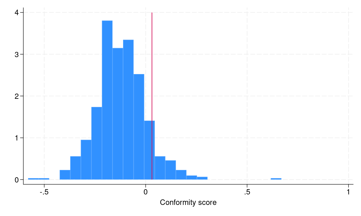
To assemble conformalized prediction intervals from step 4, we have to compute empirical quantiles eqref{eq:empquantile}, which may be executed in Stata by utilizing the _pctile command. Determine 1a exhibits the distribution of conformity scores, and the crimson vertical line signifies the empirical quantile eqref{eq:empquantile}, which is the same as 0.031.
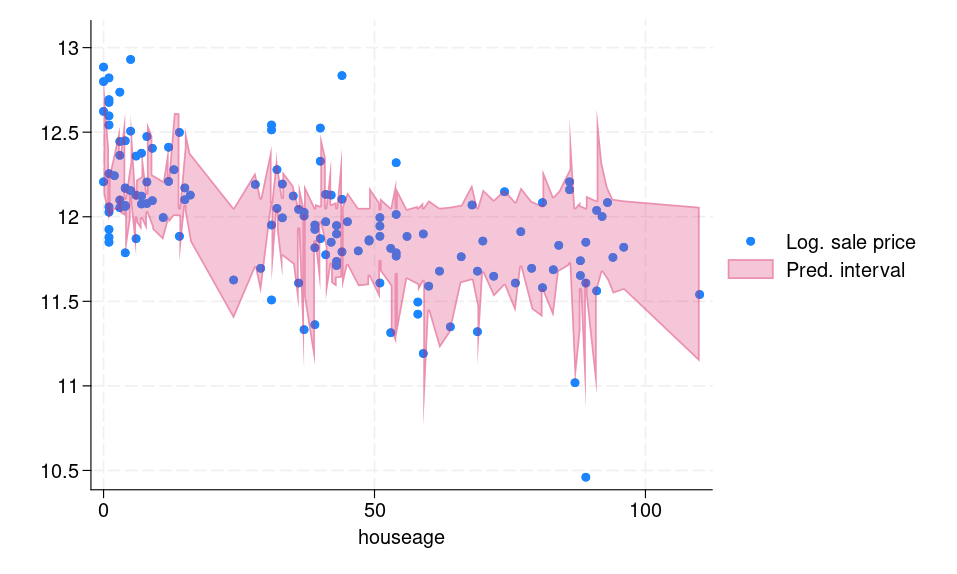
I then load these predictions from the testing body into Stata and generate decrease and higher bounds for prediction intervals. As well as, I additionally load the logsaleprice and houseage variables. We’ll use these variables for illustration functions.
Determine 1b shows the prediction intervals for every remark within the testing body. We are able to see that the computed interval is adaptive, that means for “troublesome” observations, for instance, outliers, the interval is vast and vice versa.
(a) Histogram of conformity scores
(b) Prediction intervals for the testing dataset
Determine 1: (a) Histogram of conformity scores (b) CQR-based prediction intervals for the testing dataset
Under, I record a small pattern of the prediction intervals and the true log of sale worth response.
For 9 out of 10 observations, the responses belong to the respective predictive intervals. We are able to compute the precise common protection of the interval within the testing body, which I do subsequent by producing a brand new variable, in_interval, that signifies whether or not the response logsaleprice is within the prediction interval.
We are able to see that the precise common protection is 90.5%.
References Angelopoulos, A. N., and S. Bates. 2023. Conformal prediction: A delicate introduction. Foundations and Traits in Machine Studying 16: 494–591. https://doi.org/10.1561/2200000101.
De Cock, D. 2011. Ames, Iowa: Different to the Boston housing information as an finish of semester regression mission. Journal of Statistics Training 19: 3. https://doi.org/10.1080/10691898.2011.11889627.
Lei, J., M. G’Promote, A. Rinaldo, R. J. Tibshirani, and L. Wasserman. 2018. Distribution-free predictive inference for regression. Journal of the American Statistical Affiliation 113: 1094–1111. https://doi.org/10.1080/01621459.2017.1307116.
Papadopoulos, H., Okay. Proedrou, V. Vovk, and A. Gammerman. 2002. “Inductive confidence machines for regression”. In Machine Studying: ECML 2002. Lecture Notes in Pc Science, edited by T. Elomaa, H. Mannila, H. Toivonen, vol. 2430: 345–356. Berlin: Springer. https://doi.org/10.1007/3-540-36755-1_29.
I all the time see this Google Gemini button up within the nook in Gmail. Whenever you hover over it, it does this cool animation the place the little four-pointed star spins and the outer form morphs between a pair completely different shapes which are additionally spinning.
I challenged myself to recreate the button utilizing the brand new CSS form() operate sprinkled with animation to get issues fairly shut. Let me stroll you thru it.
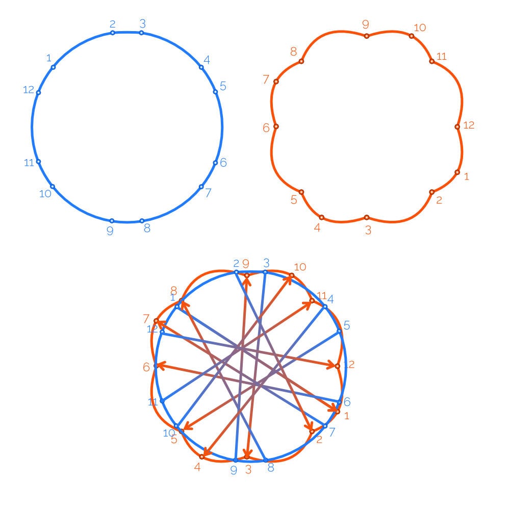
Drawing the Shapes
Breaking it down, we want 5 shapes in complete:
4-pointed star
Flower-ish factor (sure, that’s the technical time period)
Cylinder-ish factor (additionally the proper technical time period)
Rounded hexagon
Circle
I drew these shapes in a graphics enhancing program (I like Affinity Designer, however any app that allows you to draw vector shapes ought to work), outputted them in SVG, after which used a instrument, like Temani Afif’s generator, to translate the SVG paths this system generated to the CSS form() syntax.
Now, earlier than I exported the shapes from Affinity Designer, I made certain the flower, hexagon, circle, and cylinder all had the identical variety of anchor factors. In the event that they don’t have the identical quantity, then the shapes will soar from one to the following and gained’t do any morphing. So, let’s use a constant variety of anchor factors in every form — even the circle — and we are able to watch these shapes morph into one another.
I set twelve anchor factors on every form as a result of that was the very best quantity used (the hexagon had two factors close to every curved nook).
One thing associated (and presumably arduous to unravel, relying in your graphics program) is that a few of my shapes had been wildly contorted when animating between shapes. For instance, many shapes turned smaller and started spinning earlier than morphing into the following form, whereas others had been way more seamless. I finally discovered that the interpolation was matching every form’s place to begin and continued matching factors because it adopted the form.
The result’s that the matched factors transfer between shapes, so if the start line for one form is on reverse aspect of the start line of the second form, loads of motion is critical to transition from one form’s place to begin to the following form’s place to begin.
Fortunately, the circle was the one form that gave me hassle, so I used to be capable of spin it (with some trial and error) till its place to begin extra intently matched the opposite beginning factors.
One other concern I bumped into was that the cylinder-ish form had two particular person straight strains in form() with line instructions reasonably than utilizing the curve command. This prevented the animation from morphing into the following form. It instantly snapped to the following picture with out animating the transition, skipping forward to the following form (each when going into the cylinder and popping out of it).
I went again into Affinity Designer and ever-so-slightly added curvature to the 2 strains, after which it morphed completely. I initially thought this was a form() quirk, however the identical factor occurred after I tried the animation with the path() operate, suggesting it’s extra an interpolation limitation than it’s a form() limitation.
As soon as I completed including my form() values, I outlined a CSS variable for every form. This makes the later makes use of of every form() extra readable, to not point out simpler to take care of. With twelve strains per form the code is stinkin’ lengthy (technical time period) so we’ve put it behind an accordion menu.
View Form Code
:root {
  --hexagon: form(
    evenodd from 6.47% 67.001%,
    curve by 0% -34.002% with -1.1735% -7.7% / -1.1735% -26.302%,
    curve by 7.0415% -12.1965% with 0.7075% -4.641% / 3.3765% -9.2635%,
    curve by 29.447% -17.001% with 6.0815% -4.8665% / 22.192% -14.1675%,
    curve by 14.083% 0% with 4.3725% -1.708% / 9.7105% -1.708%,
    curve by 29.447% 17.001% with 7.255% 2.8335% / 23.3655% 12.1345%,
    curve by 7.0415% 12.1965% with 3.665% 2.933% / 6.334% 7.5555%,
    curve by 0% 34.002% with 1.1735% 7.7% / 1.1735% 26.302%,
    curve by -7.0415% 12.1965% with -0.7075% 4.641% / -3.3765% 9.2635%,
    curve by -29.447% 17.001% with -6.0815% 4.8665% / -22.192% 14.1675%,
    curve by -14.083% 0% with -4.3725% 1.708% / -9.7105% 1.708%,
    curve by -29.447% -17.001% with -7.255% -2.8335% / -23.3655% -12.1345%,
    curve by -7.0415% -12.1965% with -3.665% -2.933% / -6.334% -7.5555%,
    shut
  );

  --flower: form(
    evenodd from 17.9665% 82.0335%,
    curve by -12.349% -32.0335% with -13.239% -5.129% / -18.021% -15.402%,
    curve by -0.0275% -22.203% with -3.1825% -9.331% / -3.074% -16.6605%,
    curve by 12.3765% -9.8305% with 2.3835% -4.3365% / 6.565% -7.579%,
    curve by 32.0335% -12.349% with 5.129% -13.239% / 15.402% -18.021%,
    curve by 20.4535% -0.8665% with 8.3805% -2.858% / 15.1465% -3.062%,
    curve by 11.58% 13.2155% with 5.225% 2.161% / 9.0355% 6.6475%,
    curve by 12.349% 32.0335% with 13.239% 5.129% / 18.021% 15.402%,
    curve by 0.5715% 21.1275% with 2.9805% 8.7395% / 3.0745% 15.723%,
    curve by -12.9205% 10.906% with -2.26% 4.88% / -6.638% 8.472%,
    curve by -32.0335% 12.349% with -5.129% 13.239% / -15.402% 18.021%,
    curve by -21.1215% 0.5745% with -8.736% 2.9795% / -15.718% 3.0745%,
    curve by -10.912% -12.9235% with -4.883% -2.2595% / -8.477% -6.6385%,
    shut
  );

  --cylinder: form(
    evenodd from 10.5845% 59.7305%,
    curve by 0% -19.461% with -0.113% -1.7525% / -0.11% -18.14%,
    curve by 10.098% -26.213% with 0.837% -10.0375% / 3.821% -19.2625%,
    curve by 29.3175% -13.0215% with 7.2175% -7.992% / 17.682% -13.0215%,
    curve by 19.5845% 5.185% with 7.1265% 0% / 13.8135% 1.887%,
    curve by 9.8595% 7.9775% with 3.7065% 2.1185% / 7.035% 4.8195%,
    curve by 9.9715% 26.072% with 6.2015% 6.933% / 9.4345% 16.082%,
    curve by 0% 19.461% with 0.074% 1.384% / 0.0745% 17.7715%,
    curve by -13.0065% 29.1155% with -0.511% 11.5345% / -5.021% 21.933%,
    curve by -26.409% 10.119% with -6.991% 6.288% / -16.254% 10.119%,
    curve by -20.945% -5.9995% with -7.6935% 0% / -14.8755% -2.199%,
    curve by -8.713% -7.404% with -3.255% -2.0385% / -6.1905% -4.537%,
    curve by -9.7575% -25.831% with -6.074% -6.9035% / -9.1205% -15.963%,
    shut
  );

  --star: form(
    evenodd from 50% 24.787%,
    curve by 7.143% 18.016% with 0% 0% / 2.9725% 13.814%,
    curve by 17.882% 7.197% with 4.171% 4.2025% / 17.882% 7.197%,
    curve by -17.882% 8.6765% with 0% 0% / -13.711% 4.474%,
    curve by -7.143% 16.5365% with -4.1705% 4.202% / -7.143% 16.5365%,
    curve by -8.6115% -16.5365% with 0% 0% / -4.441% -12.3345%,
    curve by -16.4135% -8.6765% with -4.171% -4.2025% / -16.4135% -8.6765%,
    curve by 16.4135% -7.197% with 0% 0% / 12.2425% -2.9945%,
    curve by 8.6115% -18.016% with 4.1705% -4.202% / 8.6115% -18.016%,
    shut
  );

  --circle: form(
    evenodd from 13.482% 79.505%,
    curve by -7.1945% -12.47% with -1.4985% -1.8575% / -6.328% -10.225%,
    curve by 0.0985% -33.8965% with -4.1645% -10.7945% / -4.1685% -23.0235%,
    curve by 6.9955% -12.101% with 1.72% -4.3825% / 4.0845% -8.458%,
    curve by 30.125% -17.119% with 7.339% -9.1825% / 18.4775% -15.5135%,
    curve by 13.4165% 0.095% with 4.432% -0.6105% / 8.9505% -0.5855%,
    curve by 29.364% 16.9% with 11.6215% 1.77% / 22.102% 7.9015%,
    curve by 7.176% 12.4145% with 3.002% 3.7195% / 5.453% 7.968%,
    curve by -0.0475% 33.8925% with 4.168% 10.756% / 4.2305% 22.942%,
    curve by -7.1135% 12.2825% with -1.74% 4.4535% / -4.1455% 8.592%,
    curve by -29.404% 16.9075% with -7.202% 8.954% / -18.019% 15.137%,
    curve by -14.19% -0.018% with -4.6635% 0.7255% / -9.4575% 0.7205%,
    curve by -29.226% -16.8875% with -11.573% -1.8065% / -21.9955% -7.9235%,
    shut
  );
}
If all that appears like gobbledygook to you, it largely does to me too (and I wrote the form() Almanac entry). As I stated above, I transformed them from stuff I drew to form()s with a instrument. If you happen to can acknowledge the shapes from the customized property names, you then’ll have all it’s worthwhile to know to maintain following alongside.
Breaking Down the Animation
After staring on the Gmail animation for longer than I want to admit, I used to be capable of acknowledge six distinct phases:
First, on hover:
The four-pointed star spins to the correct and modifications shade.
The flowery blue form spreads out from beneath the star form.
The flowery blue form morphs into one other form whereas spinning.
The purplish shade is wiped throughout the flowery blue form.
Then, after hover:
The flowery blue form contracts (principally the reverse of Part 2).
The four-pointed star spins left and returns to its preliminary shade (principally the reverse of Part 1).
That’s the run sheet we’re working with! We’ll write the CSS for all that in a bit, however first I’d wish to arrange the HTML construction that we’re hooking into.
The HTML
I’ve all the time needed to be a kind of front-enders who make jaw-dropping artwork out of CSS, like illustrating the Sistine chapel ceiling with a single div (cue somebody commenting with a CodePen doing simply that). However, alas, I made a decision I wanted two divs to perform this problem, and I thanks for wanting previous my disgrace. To these of you who turned up your nostril and stopped studying after that admission: I can safely name you a Flooplegerp and also you’ll by no means understand it.
(To these of you continue to with me, I don’t truly know what a Flooplegerp is. However I’m certain it’s unhealthy.)
As a result of the animation must unfold out the blue form from beneath the star form, they must be two separate shapes. And we are able to’t shrink or clip the primary ingredient to do that as a result of that may obscure the star.
So, yeah, that’s why I’m reaching for a second div: to deal with the flowery form and the way it wants to maneuver and work together with the star form.
The Fundamental CSS Styling
Every form is basically outlined with the identical field with the identical dimensions and margin spacing.
We are able to clip the field to a selected form utilizing a pseudo-element. For instance, let’s clip a star form utilizing the CSS variable (--star) we outlined for it and set a background shade on it:
We are able to hook into the container’s youngster div and use it to determine the animation’s beginning form, which is the flower (clipped with our --flower variable):
What we get is a star form stacked proper on high of a flower form. We’re virtually carried out with our preliminary CSS, however with the intention to recreate the animated shade wipes, we want a a lot bigger floor that permits us to “change” colours by shifting the background gradient’s place. Let’s transfer the gradient in order that it's declared on a pseudo ingredient as an alternative of the kid div, and dimension it up by 400% to provide us extra respiration room.
Now we are able to clearly see how the shapes are positioned relative to one another:
Animating Phases 1 and 6
Now, I’ll admit, in my very own hubris, I’ve turned up my very personal schnoz on the humble transition property as a result of my considering is usually, Transitions are nice for getting began in animation and for fast issues, however actual animations are carried out with CSS keyframes. (Maybe I, too, am a Flooplegerp.)
However now I see the error of my methods. I can write a set of keyframes that rotate the star 180 levels, flip its shade white(ish), and have it keep that means for so long as the ingredient is hovered. What I can’t do is animate the star again to what it was when the ingredient is un-hovered.
I can, nonetheless, try this with the transition property. To do that, we add transition: 1s ease-in-out; on the ::earlier than, including the brand new background shade and rotating issues on :hover over the #geminianimation container. This accounts for the primary and sixth phases of the animation we outlined earlier.
We are able to do one thing comparable for the second and fifth phases of the animation since they're mirror reflections of one another. Keep in mind, in these phases, we’re spreading and contracting the flowery blue form.
We are able to begin by shrinking the interior div’s scale to zero initially, then broaden it again to its authentic dimension (scale: 1) on :hover (once more utilizing transitions):
#geminianimation {
  div {
    scale: 0;
    transition: 1s ease-in-out;
  }
  &:hover {
    div {
      scale: 1;
  }
}
Animating Part 3
Now, we very properly may deal with this with a transition like we did the final two units, however we most likely shouldn't do it… that's, until you wish to weep bitter tears and curse the day you first heard of CSS… not that I do know from private expertise or something… ha ha… ha.
CSS keyframes are a greater match right here as a result of there are a number of states to animate between that may require defining and orchestrating a number of completely different transitions. Keyframes are more proficient at tackling multi-step animations.
What we’re principally doing is animating between completely different shapes that we’ve already outlined as CSS variables that clip the shapes. The browser will deal with interpolating between the shapes, so all we want is to inform CSS which form we would like clipped at every part (or “part”) of this set of keyframes:
Sure, we may mix the primary and final keyframes (0% and 100%) right into a single step, however we’ll want them separated in a second as a result of we additionally wish to animate the rotation on the similar time. We’ll set the preliminary rotation to 0turn and the ultimate rotation 1turn in order that it may possibly hold spinning easily so long as the animation is continuous:
Word: Sure, flip is certainly a CSS unit, albeit one that usually goes missed.
We wish the animation to be easy because it interpolates between shapes. So, I’m setting the animation’s timing operate with ease-in-out. Sadly, this may also decelerate the rotation because it begins and ends. Nevertheless, as a result of we’re each starting and ending with the circle form, the truth that the rotation slows popping out of 0% and slows once more because it heads into 100% isn't noticeable — a circle seems to be like a circle regardless of its rotation. If we had been ending with a unique form, the easing can be seen and I'd use two separate units of keyframes — one for the shape-shift and one for the rotation — and name them each on the #geminianimation youngster div .
That stated, we nonetheless do want yet one more set of keyframes, particularly for altering the form’s shade. Keep in mind how we set a linear gradient on the mum or dad container’s ::after pseudo, then we additionally elevated the pseudo’s width and top? Right here’s that little bit of code once more:
The gradient is that giant as a result of we’re solely displaying a part of it at a time. And which means we are able to translate the gradient’s place to maneuver the gradient at sure keyframes. 400% could be properly divided into quarters, so we are able to transfer the gradient by, say, three-quarters of its dimension. Since its mum or dad, the #geminianimation div, is already spinning, we don’t want any fancy actions to make it really feel like the colour is coming from completely different instructions. We simply translate it linearly and the spin provides some variability to what route the colour wipe comes from.
As a substitute of utilizing the flower because the default form, let’s change it to circle. This smooths issues out when the hover interplay causes the animation to cease and return to its preliminary place.
And there you've it:
Wrapping up
We did it! Is that this precisely how Google completed the identical factor? In all probability not. In all honesty, I by no means inspected the animation code as a result of I needed to strategy it from a clear slate and work out how I'd do it purely in CSS.
That’s the enjoyable factor a couple of problem like this: there are alternative ways to perform the identical factor (or one thing comparable), and your means of doing it's prone to be completely different than mine. It’s enjoyable to see a wide range of approaches.
Which leads me to ask: How would you've approached the Gemini button animation? What concerns would you consider that perhaps I haven’t?
It’s been some time since I final posted a brand new entry on the TorchVision memoirs collection. Thought, I’ve beforehand shared information on the official PyTorch weblog and on Twitter, I assumed it might be a good suggestion to speak extra about what occurred on the final launch of TorchVision (v0.12), what’s popping out on the subsequent one (v0.13) and what are our plans for 2022H2. My goal is to transcend offering an summary of recent options and quite present insights on the place we wish to take the venture within the following months.
TorchVision v0.12 was a large launch with twin focus: a) replace our deprecation and mannequin contribution insurance policies to enhance transparency and entice extra group contributors and b) double down on our modernization efforts by including well-liked new mannequin architectures, datasets and ML strategies.
Updating our insurance policies
Key for a profitable open-source venture is sustaining a wholesome, energetic group that contributes to it and drives it forwards. Thus an essential purpose for our group is to extend the variety of group contributions, with the long run imaginative and prescient of enabling the group to contribute huge options (new fashions, ML strategies, and many others) on prime of the standard incremental enhancements (bug/doc fixes, small options and many others).
Traditionally, although the group was keen to contribute such options, our group hesitated to just accept them. Key blocker was the dearth of a concrete mannequin contribution and deprecation coverage. To deal with this, Joao Gomes labored with the group to draft and publish our first mannequin contribution pointers which offers readability over the method of contributing new architectures, pre-trained weights and options that require mannequin coaching. Furthermore, Nicolas Hug labored with PyTorch core builders to formulate and undertake a concrete deprecation coverage.
The aforementioned modifications had speedy constructive results on the venture. The brand new contribution coverage helped us obtain quite a few group contributions for big options (extra particulars beneath) and the clear deprecation coverage enabled us to scrub up our code-base whereas nonetheless guaranteeing that TorchVision presents robust Backwards Compatibility ensures. Our group may be very motivated to proceed working with the open-source builders, analysis groups and downstream library creators to take care of TorchVision related and contemporary. When you’ve got any suggestions, remark or a characteristic request please attain out to us.
Modernizing TorchVision
It’s no secret that for the previous few releases our goal was so as to add to TorchVision all the required Augmentations, Losses, Layers, Coaching utilities and novel architectures in order that our customers can simply reproduce SOTA outcomes utilizing PyTorch. TorchVision v0.12 continued down that route:
Our rockstar group contributors, Hu Ye and Zhiqiang Wang, have contributed the FCOS structure which is a one-stage object detection mannequin.
Nicolas Hug has added assist of optical move in TorchVision by including the RAFT structure.
As per standard, the discharge got here with quite a few smaller enhancements, bug fixes and documentation enhancements. To see the entire new options and the record of our contributors please verify the v0.12 launch notes.
TorchVision v0.13 is simply across the nook, with its anticipated launch in early June. It’s a very huge launch with a major variety of new options and massive API enhancements.
Wrapping up Modernizations and shutting the hole from SOTA
We’re persevering with our journey of modernizing the library by including the required primitives, mannequin architectures and recipe utilities to supply SOTA outcomes for key Pc Imaginative and prescient duties:
With the assistance of Victor Fomin, I’ve added essential lacking Information Augmentation strategies equivalent to AugMix, Giant Scale Jitter and many others. These strategies enabled us to shut the hole from SOTA and produce higher weights (see beneath).
With the assistance of Aditya Oke, Hu Ye, Yassine Alouini and Abhijit Deo, we’ve added essential widespread constructing blocks such because the DropBlock layer, the MLP block, the cIoU & dIoU loss and many others. Lastly I labored with Shen Li to repair a protracted standing situation on PyTorch’s SyncBatchNorm layer which affected the detection fashions.
Hu Ye with the assist of Joao Gomes added Swin Transformer together with improved pre-trained weights. I added the EfficientNetV2 structure and a number of other post-paper architectural optimizations on the implementation of RetinaNet, FasterRCNN and MaskRCNN.
As I mentioned earlier on the PyTorch weblog, we’ve put vital effort on enhancing our pre-trained weights by creating an improved coaching recipe. This enabled us to enhance the accuracy of our Classification fashions by 3 accuracy factors, attaining new SOTA for numerous architectures. The same effort was carried out for Detection and Segmentation, the place we improved the accuracy of the fashions by over 8.1 mAP on common. Lastly Yosua Michael M labored with Laura Gustafson, Mannat Singhand and Aaron Adcock so as to add assist of SWAG, a set of recent extremely correct state-of-the-art pre-trained weights for ViT and RegNets.
New Multi-weight assist API
As I beforehand mentioned on the PyTorch weblog, TorchVision has prolonged its current mannequin builder mechanism to assist a number of pre-trained weights. The brand new API is totally backwards appropriate, permits to instantiate fashions with completely different weights and offers mechanisms to get helpful meta-data (equivalent to classes, variety of parameters, metrics and many others) and the preprocessing inference transforms of the mannequin. There’s a devoted suggestions situation on Github to assist us iron our any tough edges.
Revamped Documentation
Nicolas Hug led the efforts of restructuring the mannequin documentation of TorchVision. The brand new construction is ready to make use of options coming from the Multi-weight Assist API to supply a greater documentation for the pre-trained weights and their use within the library. Huge shout out to our group members for serving to us doc all architectures on time.
Thought our detailed roadmap for 2022H2 shouldn’t be but finalized, listed here are some key tasks that we’re at the moment planing to work on:
Philip Meier and Nicolas Hug are engaged on an improved model of the Datasets API (v2) which makes use of TorchData and Information pipes. Philip Meier, Victor Fomin and I are additionally engaged on extending our Transforms API (v2) to assist not solely photographs but additionally bounding containers, segmentation masks and many others.
Lastly the group helps us preserve TorchVision contemporary and related by including well-liked architectures and strategies. Lezwon Castelino is at the moment working with Victor Fomin so as to add the SimpleCopyPaste augmentation. Hu Ye is at the moment working so as to add the DeTR structure.
If you need to become involved with the venture, please take a look to our good first points and the assist wished lists. In case you are a seasoned PyTorch/Pc Imaginative and prescient veteran and also you want to contribute, we’ve a number of candidate tasks for brand new operators, losses, augmentations and fashions.
I hope you discovered the article attention-grabbing. If you wish to get in contact, hit me up on LinkedIn or Twitter.
AI Adoption in enterprises is a no brainer. Shouldn’t everybody be on it by now? You’ll suppose so. Companies which have adopted it efficiently are acing it. Predictive analytics, sensible automation, and knowledgeable decision-making are a breeze for them.
For just a few, nonetheless, AI adoption in enterprises continues to be patchy. Most corporations have success in proof-of-concepts however fail to copy them. In recent times, extra companies have seen the necessity to discard AI tasks earlier than manufacturing.
That’s why this weblog talks about essentially the most vital challenges in AI adoption, and the way companies can overcome them. Learn on!
Uncover How Your Enterprise Can Harness AI For Most Affect
Greater than three-quarters (78%) of companies apply AI in a number of enterprise processes. Whereas CEOs all concur that AI is the long run, many discover that scaling past pilots is difficult. Problem in cross-department collaboration, expertise hole, unclear ROI, and safety points are some causes.
Right here is an outline of the principle the explanation why corporations are having bother making use of AI:
Knowledge Complexity and Silos : AI fashions rely upon knowledge high quality. But, 72% of enterprises admit their AI purposes are developed in silos with out cross-department collaboration. This fragmentation reduces accuracy and scalability.
Expertise and Abilities Hole: AI adoption calls for knowledge scientists, ML engineers, and area consultants. However 70% of senior leaders say their workforce isn’t able to leverage AI successfully.
Excessive Prices and Unclear ROI: Enterprises hesitate when infrastructure, integration, and hiring prices overshadow speedy returns. In truth, solely 17% of corporations attribute 5% or extra of their EBIT to AI initiatives.
Organizational Resistance to Change: Worker resistance is a significant problem. 45% of CEOs say their workers are resistant and even brazenly hostile to AI.
Safety, Privateness, and Points with Compliance: AI consumes delicate knowledge. On account of this, abiding by legal guidelines like GDPR turns into tough. Missing efficient governance, corporations are apprehensive about repute harm and penalties.
A Look into the Dangers and Blockers of Scaling AI Throughout Organizations
Even when pilots succeed, enterprises face limitations in scaling AI throughout the group. The important thing issue is the lack of information of the way in which AI fashions function. Mannequin drifts that scale back accuracy, integration challenges, and value overruns are some causes that might impede scaling. Let’s have a look at some key dangers and blockers of AI adoption in enterprises:
1. Shadow AI and Rogue Initiatives
Departments begin “shadow AI” tasks with little IT governance. Native success interprets to enterprise-wide failure, forming silos, duplication, and the hazard of non-compliance.
2. Mannequin Drift and Upkeep Burden
AI fashions are degrading over time with altering market developments and consumer habits. Enterprises don’t know the worth of ongoing monitoring and retraining. This leads to “mannequin drift,” which reduces accuracy and reliability. Poorly skilled fashions might amplify biases, risking reputational and authorized challenges.
3. Lack of Interoperability Requirements
With extra AI platforms rising, corporations battle interoperability. They’re usually hampered by integration challenges in scaling AI owing to variable knowledge codecs and incompatible programs.
4. The Hidden Prices of Scaling Infrastructure
Scaling AI doesn’t take simply algorithms. There’s extra behind the scenes. Cloud storage, GPU computing energy, and safety controls value cash. Most corporations underestimate these hidden bills, resulting in value overruns.
5. Cultural Misalignment Between Enterprise and IT
Profitable AI calls for cross-functional alignment. IT is apprehensive about safety and compliance, and enterprise models are at all times in a rush. The conflict of cultures will get in the way in which of execution and retains enterprise-wide scaling at bay.
Suggestions To Overcome These Challenges
AI adoption challenges in enterprises are widespread. However that doesn’t imply that they aren’t not possible to beat. Listed here are some tricks to velocity up AI adoption in enterprises:
Set up Crystal Clear Enterprise Objectives: AI should handle enterprise priorities, not merely undertake know-how for the sake of it. Leaders want to find out high-impact alternatives. Fraud detection, customer support automation, and demand forecasting are priorities.
Spend money on Knowledge Readiness : Excessive-quality, built-in knowledge is vital. Enterprises require good governance and built-in knowledge in real-time. Organized knowledge habits are much more prone to derive ROI from AI.
Manage Cross-Practical Groups :AI is greatest with IT, enterprise, regulatory, and area subject material consultants in collaboration. It allows scalability and reduces moral threat.
Upskill and Reskill Expertise: Cultural readiness is required for AI deployment. Solely 14% of organizations had a very synchronized workforce, know-how, and development technique—the “AI pacesetters”. Studying investments stop extra transition issues.
Pilot Small, Scale Quick: Pilot tasks should produce quantifiable ROI earlier than large-scale adoption. This instills organizational confidence and reduces monetary threat.
Emphasize AI Governance and Ethics: Open fashions, bias testing, and compliance frameworks set up worker and buyer belief.
Collaborate with Seasoned Suppliers: Firms that lack in-house experience deliver worth by partnering with seasoned AI suppliers like Fingent, that are centered on filling ability gaps, managing integration, and scaling responsibly.
Standard FAQs Associated to AI Adoption in Enterprises
Q1: What are the principle limitations to AI adoption in enterprises?
The first inhibitors of AI adoption in enterprises are siloed knowledge. The absence of competent expertise, obscure ROI, cultural opposition, and governance are just a few different elements that pose challenges in AI adoption.
Q2: Why do AI pilots work however get caught on scaling?
This occurs as a result of scaling wants sturdy knowledge programs, governance, and alignment at departmental ranges. With out them, pilots don’t work in manufacturing.
Q3: How can companies overcome AI adoption challenges?
AI adoption challenges in enterprises might be overcome for those who first set clear enterprise goals. As soon as that’s completed, spend money on upskilling workers and partnering up with seasoned AI suppliers like Fingent.
This autumn: Is AI adoption in enterprises well worth the dangers?
Sure! Greatest-practice adopting corporations usually tend to see constructive returns and ROI. However corporations with no AI technique witness enterprise success solely 37% of the time. Whereas corporations with a minimum of one AI implementation mission succeed 80% of the time.
Q5: That are the industries that profit most from AI adoption?
Tech appears to return instantly to thoughts. However the previous few years have seen different industries jostle for house on the highest listing of adopters. The pharmaceutical business has found what AI can do for scientific trials. Chatbots and digital assistants have revolutionized banking and retail. Predictive upkeep has smoothed out many an issue for the manufacturing business.
Strategize a Clean AI Transition. We Can Assist You Effortlessly Combine AI into Your Present Techniques
How Can Fingent Assist?
At Fingent, we cope with the intricacies of AI implementation in enterprise organizations regularly. Our capabilities are:
Scalable AI answer planning based mostly on enterprise goals.
Efficient knowledge governance fashions.
Glitch-free integration with legacy programs.
Moral and clear AI mannequin constructing.
Cultural transformation via adoption and upskilling initiatives.
Whether or not what you are promoting is simply beginning pilots or preventing to scale, Fingent can help in optimizing ROI and mitigating dangers. Study extra about our AI companies right here.
Knock These Limitations With Us
AI adoption limitations in enterprise nonetheless hold organizations from realizing potential. The silver lining? With the fitting technique and partnerships, companies can blow previous the challenges and drive a profitable AI adoption journey.
The way forward for AI adoption in enterprises is just not algorithms; it’s about belief, collaboration, and a imaginative and prescient for the long term. Those that act at this time will reign supreme tomorrow. Give us a name and let’s knock these limitations down and lead what you are promoting to creating a hit of AI.
Knowledge has change into an indispensable useful resource for any profitable enterprise, because it offers beneficial insights for knowledgeable decision-making. Given the significance of information, many firms are constructing techniques to retailer and analyze it. Nevertheless, there are various occasions when it’s laborious to accumulate and analyze the required information, particularly with the growing complexity of the information system.
With the arrival of generative AI, information work has change into considerably simpler, as we are able to now use easy pure language to obtain principally correct output that intently follows the enter we offer. It’s additionally relevant to information processing and evaluation with SQL, the place we are able to ask for question improvement.
On this article, we are going to develop a easy API software that interprets pure language into SQL queries that our database understands. We are going to use three principal instruments: OpenAI, FastAPI, and SQLite.
Right here’s the plan.
# Textual content-to-SQL App Growth
First, we’ll put together all the things wanted for our mission. All it is advisable present is the OpenAI API key, which we’ll use to entry the generative mannequin. To containerize the appliance, we are going to use Docker, which you’ll purchase for the native implementation utilizing Docker Desktop.
Different elements, similar to SQLite, will already be accessible once you set up Python, and FastAPI will likely be put in later.
For the general mission construction, we are going to use the next:
Create the construction like above, or you need to use the next repository to make issues simpler. We are going to nonetheless undergo every file to realize an understanding of how you can develop the appliance.
Let’s begin by populating the .env file with the OpenAI API key we beforehand acquired. You are able to do that with the next code:
OPENAI_API_KEY=YOUR-API-KEY
Then, go to the necessities.txt to fill within the crucial libraries we are going to use for
Subsequent, we transfer on to the __init__.py file, and we are going to put the next code inside:
from pathlib import Path
from dotenv import load_dotenv

load_dotenv(dotenv_path=Path(__file__).resolve().father or mother.father or mother / ".env", override=False)
The code above ensures that the atmosphere comprises all the required keys we want.
Then, we are going to develop Python code within the database.py file to connect with the SQLite database we are going to create later (referred to asdemo.db) and supply a solution to run SQL queries.
from sqlalchemy import create_engine, textual content
from sqlalchemy.orm import Session

ENGINE = create_engine("sqlite:///demo.db", future=True, echo=False)

def run_query(sql: str) -> listing[dict]:
    with Session(ENGINE) as session:
        rows = session.execute(textual content(sql)).mappings().all()
    return [dict(r) for r in rows]
After that, we are going to put together the openai_utils.py file that can settle for the database schema and the enter questions. The output will likely be JSON containing the SQL question (with a guard to stop any write operations).
import os
import json
from openai import OpenAI

shopper = OpenAI(api_key=os.getenv("OPENAI_API_KEY"))

_SYSTEM_PROMPT = """
You change natural-language questions into read-only SQLite SQL.
By no means output INSERT / UPDATE / DELETE.
Return JSON: { "sql": "..." }.
"""

def text_to_sql(query: str, schema: str) -> str:
    response = shopper.chat.completions.create(
        mannequin="gpt-4o-mini",
        temperature=0.1,
        response_format={"kind": "json_object"},
        messages=[
            {"role": "system", "content": _SYSTEM_PROMPT},
            {"role": "user",
             "content": f"schema:n{schema}nnquestion: {question}"}
        ]
    )
    payload = json.hundreds(response.selections[0].message.content material)
    return payload["sql"]
With each the code and the connection prepared, we are going to put together the appliance utilizing FastAPI. The applying will settle for pure language questions and the database schema, convert them into SQL SELECT queries, run them by means of the SQLite database, and return the outcomes as JSON. The applying will likely be an API we are able to entry by way of the CLI.
from fastapi import FastAPI, HTTPException
from pydantic import BaseModel
from sqlalchemy import examine
from .database import ENGINE, run_query
from .openai_utils import text_to_sql

app = FastAPI(title="Textual content-to-SQL Demo")

class NLRequest(BaseModel):
    query: str

@app.on_event("startup")
def capture_schema() -> None:
    insp = examine(ENGINE)
    international SCHEMA_STR
    SCHEMA_STR = "n".be part of(
        f"CREATE TABLE {t} ({', '.be part of(c['name'] for c in insp.get_columns(t))});"
        for t in insp.get_table_names()
    )

@app.submit("/question")
def question(req: NLRequest):
    attempt:
        sql = text_to_sql(req.query, SCHEMA_STR)
        if not sql.lstrip().decrease().startswith("choose"):
            increase ValueError("Solely SELECT statements are allowed")
        return {"sql": sql, "consequence": run_query(sql)}
    besides Exception as e:
        increase HTTPException(status_code=400, element=str(e))
That’s all the things we want for the primary software. The subsequent factor we are going to put together is the database. Use the database under within the init_db.sql for instance functions, however you may at all times change it if you’d like.
DROP TABLE IF EXISTS order_items;
DROP TABLE IF EXISTS orders;
DROP TABLE IF EXISTS funds;
DROP TABLE IF EXISTS merchandise;
DROP TABLE IF EXISTS prospects;

CREATE TABLE prospects (
    id INTEGER PRIMARY KEY,
    title TEXT NOT NULL,
    nation TEXT,
    signup_date DATE
);

CREATE TABLE merchandise (
    id INTEGER PRIMARY KEY,
    title TEXT NOT NULL,
    class TEXT,
    value REAL
);

CREATE TABLE orders (
    id INTEGER PRIMARY KEY,
    customer_id INTEGER,
    order_date DATE,
    complete REAL,
    FOREIGN KEY (customer_id) REFERENCES prospects(id)
);

CREATE TABLE order_items (
    order_id INTEGER,
    product_id INTEGER,
    amount INTEGER,
    unit_price REAL,
    PRIMARY KEY (order_id, product_id),
    FOREIGN KEY (order_id) REFERENCES orders(id),
    FOREIGN KEY (product_id) REFERENCES merchandise(id)
);

CREATE TABLE funds (
    id INTEGER PRIMARY KEY,
    order_id INTEGER,
    payment_date DATE,
    quantity REAL,
    methodology TEXT,
    FOREIGN KEY (order_id) REFERENCES orders(id)
);

INSERT INTO prospects (id, title, nation, signup_date) VALUES
 (1,'Alice','USA','2024-01-05'),
 (2,'Bob','UK','2024-03-10'),
 (3,'Choi','KR','2024-06-22'),
 (4,'Dara','ID','2025-01-15');

INSERT INTO merchandise (id, title, class, value) VALUES
 (1,'Laptop computer Professional','Electronics',1500.00),
 (2,'Noise-Canceling Headphones','Electronics',300.00),
 (3,'Standing Desk','Furnishings',450.00),
 (4,'Ergonomic Chair','Furnishings',250.00),
 (5,'Monitor 27"','Electronics',350.00);

INSERT INTO orders (id, customer_id, order_date, complete) VALUES
 (1,1,'2025-02-01',1850.00),
 (2,2,'2025-02-03',600.00),
 (3,3,'2025-02-05',350.00),
 (4,1,'2025-02-07',450.00);

INSERT INTO order_items (order_id, product_id, amount, unit_price) VALUES
 (1,1,1,1500.00),
 (1,2,1,300.00),
 (1,5,1,350.00),
 (2,3,1,450.00),
 (2,4,1,250.00),
 (3,5,1,350.00),
 (4,3,1,450.00);

INSERT INTO funds (id, order_id, payment_date, quantity, methodology) VALUES
 (1,1,'2025-02-01',1850.00,'Credit score Card'),
 (2,2,'2025-02-03',600.00,'PayPal'),
 (3,3,'2025-02-05',350.00,'Credit score Card'),
 (4,4,'2025-02-07',450.00,'Financial institution Switch');
Then, run the next code in your CLI to create a SQLite database for our mission.
sqlite3 demo.db < init_db.sql
With the database prepared, we are going to create a Dockerfile to containerize our software.
FROM python:3.12-slim
WORKDIR /code

COPY necessities.txt .
RUN pip set up --no-cache-dir -r necessities.txt

COPY . .

CMD ["uvicorn", "app.main:app", "--host", "0.0.0.0", "--port", "8000"]
We can even create a docker-compose.yml file for working the appliance extra easily.
With all the things prepared, begin your Docker Desktop and run the next code to construct the appliance.
docker compose construct --no-cache
docker compose up -d
If all the things is completed nicely, you may take a look at the appliance by utilizing the next code. We are going to ask what number of prospects now we have within the information.
curl -X POST "http://localhost:8000/question" -H "Content material-Sort: software/json" -d "{"query":"What number of prospects?"}"
The output will appear to be this.
{"sql":"SELECT COUNT(*) AS customer_count FROM prospects;","consequence":[{"customer_count":4}]}
We are able to attempt one thing extra complicated, just like the variety of orders for every buyer:
curl -X POST "http://localhost:8000/question" -H "Content material-Sort: software/json" -d "{"query":"What's the variety of orders positioned by every buyer"}"
With output like under.
{"sql":"SELECT customer_id, COUNT(*) AS number_of_orders FROM orders GROUP BY customer_id;","consequence":[{"customer_id":1,"number_of_orders":2},{"customer_id":2,"number_of_orders":1},{"customer_id":3,"number_of_orders":1}]}
That’s all it is advisable construct a fundamental Textual content-to-SQL software. You may improve it additional with a front-end interface and a extra complicated system tailor-made to your wants.
# Wrapping Up
Knowledge is the center of any information work, and corporations use it to make choices. Many occasions, the system now we have is just too complicated, and we have to depend on generative AI to assist us navigate it.
On this article, now we have discovered how you can develop a easy Textual content-to-SQL software utilizing the OpenAI mannequin, FastAPI, and SQLite.
I hope this has helped!
Cornellius Yudha Wijaya is a knowledge science assistant supervisor and information author. Whereas working full-time at Allianz Indonesia, he likes to share Python and information suggestions by way of social media and writing media. Cornellius writes on a wide range of AI and machine studying subjects.
AT&T customers are reporting that the service is down.
It seems the reviews started as early as this morning, however now the reviews are spiking.
Replace: October 17, 2025 (7:58 PM ET): After a short outage, it seems that AT&T’s community is beginning to return to regular.
Authentic article: October 17, 2025 (5:17 PM ET): For those who’re an AT&T buyer and also you’re having hassle with the service, you’re not alone. A rising variety of customers are reporting that the community is experiencing an outage.
Don’t need to miss the very best from Android Authority?
Over on DownDetector, it seems that reviews of an outage began coming in as early as this morning. Nevertheless, the quantity by no means received larger than 600 reviews, and it began to dip at round 2:00 PM ET. Now that quantity has all of the sudden spiked to round 1,700 and it seems to be just like the variety of reviews are nonetheless climbing.
In keeping with the web page, the best variety of reviews are coming from cities, like Atlanta, Charlotte, Miami, Dallas, Nashville, and extra. We’ll be keeping track of the state of affairs because it develops. We’ll replace this text when indicators are exhibiting that AT&T is again up and operating.
Thanks for being a part of our group. Learn our Remark Coverage earlier than posting.
The integrity of a dissertation’s findings closely depends on the suitable utility of statistical checks. T-tests, like different parametric checks, are constructed upon a set of assumptions in regards to the information. If these assumptions are considerably violated, the outcomes generated by the t-test (such because the p-value and confidence intervals) could also be inaccurate, probably resulting in faulty conclusions and jeopardizing the dissertation’s credibility. Due to this fact, understanding and checking these assumptions shouldn’t be merely a procedural hurdle however a crucial step in safeguarding the validity of the analysis.
Core T-Take a look at Assumptions Defined:
Normality: The information for the dependent variable inside every group (for impartial samples t-tests) or the distribution of the variations between paired observations (for paired samples t-tests) ought to be roughly usually distributed.
Pupil Problem & Resolution: A standard query is, “How do I verify this?” Normality may be assessed visually utilizing histograms or Q-Q plots, or statistically utilizing checks just like the Shapiro-Wilk take a look at or Kolmogorov-Smirnov take a look at. It is very important notice that t-tests are comparatively strong to minor violations of normality, particularly with bigger pattern sizes.
Homogeneity of Variances (Equality of Variances): This assumption applies particularly to the impartial samples t-test and requires that the variances of the dependent variable are equal throughout the 2 teams being in contrast.
Pupil Problem & Resolution: “What if the variances aren’t equal?” Levene’s take a look at is usually used to verify this assumption. If Levene’s take a look at is important (indicating unequal variances), an alternate model of the t-test, resembling Welch’s t-test, ought to be used because it doesn’t assume equal variances.
Need assistance conducting your T-Take a look at? Leverage our 30+ years of expertise and low-cost same-day service to finish your outcomes at the moment!
Independence of Observations: The observations inside every group should be impartial of one another, and if evaluating two teams, the teams themselves should be impartial (for the impartial samples t-test). For paired samples t-tests, the pairs are dependent, however particular person pairs ought to be impartial of different pairs.
Pupil Problem & Resolution: “How do I guarantee this?” This assumption is primarily addressed by means of sound analysis design and information assortment procedures, resembling random sampling or random project to teams, and making certain that one participant’s responses don’t affect one other’s.
Degree of Measurement: The dependent variable (the result being measured) ought to be steady, that means it’s measured on an interval or ratio scale. The impartial variable, which defines the teams or situations, ought to be categorical (nominal or ordinal) and, for traditional t-tests, have precisely two ranges or classes.
It’s common for real-world dissertation information to not completely meet all assumptions. College students usually surprise, “What if my information violates these assumptions?” Fortuitously, minor deviations, notably with sufficient pattern sizes, could not severely compromise the t-test outcomes. Nonetheless, for extra substantial violations, options ought to be thought-about:
Non-parametric checks: If the normality assumption is significantly violated, particularly with small samples, non-parametric options just like the Mann-Whitney U take a look at (for impartial samples) or the Wilcoxon signed-rank take a look at (for paired samples) can be utilized. These checks don’t depend on the idea of usually distributed information.
Welch’s t-test: As talked about, if the homogeneity of variances assumption is violated in an impartial samples t-test, Welch’s t-test supplies a extra dependable end result.
Statistical software program may be invaluable on this course of. For example, Intellectus Statistics simplifies this significant step by routinely checking these assumptions when a t-test is chosen. If assumptions are violated, the software program may even recommend or run applicable non-parametric equal checks, thereby eradicating a lot of the guesswork and potential for error. This performance transforms a posh diagnostic process right into a extra manageable a part of the evaluation, permitting college students to proceed with higher confidence within the appropriateness of their chosen statistical methodology. Addressing these “what if” situations proactively empowers college students and reduces the nervousness related to the technical facets of statistical evaluation


