On the Galaxy Unpacked occasion in February 2026, Samsung and Google showcased a characteristic that permits Gemini to deal with duties in your behalf. In case you are unfamiliar with it, Gemini display screen automation will help with actions like ordering meals, calling a cab, or inserting grocery orders with out you touching your telephone.
Quickly after the Galaxy S26 sequence went on sale earlier this month, Samsung started rolling out the characteristic within the U.S. and Korea. Our editor Nick Sutrich tried it hands-on and described it as “subsequent degree automation”
Article continues under
And now, the characteristic can also be arriving on the Pixel 10 sequence within the U.S. As noticed by 9to5Google first, the characteristic now accessible throughout your entire lineup, together with the Pixel 10, Pixel 10 Professional, Pixel 10 Professional XL, and Pixel 10 Professional Fold working Android 16 QPR3 steady.
(Picture credit score: Android Central)
You’ll set off the characteristic the identical method you entry Gemini now, both by holding the ability button or utilizing the “Hey Google” command. As soon as activated, Gemini walks by way of the duty step-by-step on display screen in a digital window, displaying what it’s doing, and you’ll take management at any time. It additionally asks for ultimate affirmation earlier than finishing the motion.
Customers can discover the characteristic within the Gemini app settings below Display screen automation. For now, it helps a restricted set of apps, together with Lyft, Uber, Uber Eats, Grubhub, DoorDash, and Starbucks. Gemini can even ask follow-up questions, corresponding to deciding on a drink measurement or retailer location when inserting an order.
The report additionally notes that utilization limits rely in your Gemini subscription tier. Free customers could make round 5 requests per day, whereas Gemini Extremely subscribers can go as much as 120 requests every day. .
Get the newest information from Android Central, your trusted companion on the planet of Android
Android Central’s Take
It is nice to see this characteristic arriving on extra Android telephones now. This type of automation is what agentic AI has been about, and we’re lastly seeing it in motion throughout a number of telephone fashions. I simply can not watch for Google to roll it out to extra areas as nicely.
Sharks off the coast of the Bahamas are entering into medicine like cocaine, caffeine and painkillers — or fairly, medicine are entering into them. The contaminated blood of species together with nurse sharks and Caribbean reef sharks reveals the harm people have completed to paradisiac oceanic environments.
“We’re speaking a couple of very distant island within the Bahamas,” says Natascha Wosnick, a biologist with the Federal College of Paraná in Brazil.
Wosnick is a part of a workforce that has analyzed pollution in sharks within the Caribbean and Brazil. In earlier analysis, they discovered cocaine and uncommon earth components in sharks off Rio de Janeiro.
For a brand new examine, revealed within the Might Environmental Air pollution, the workforce analyzed blood from 85 sharks captured round Eleuthera Island within the Bahamas, testing for practically two dozen authorized and unlawful medicine. Twenty-eight sharks from three species had caffeine, anti-inflammatory painkillers or different medicine of their blood. Some examined optimistic for a number of medicine. Caffeine was the commonest, adopted by acetaminophen and diclofenac, the lively substances in Tylenol and Voltaren.
Most sharks had been caught about 4 miles offshore, round an inactive fish farm in style with divers. Wosnick says currents may carry drug traces from sewage or different sources on the island, however divers are the extra doubtless culprits. “It’s principally as a result of individuals are going there, peeing within the water and dumping their sewage within the water,” she says.
Researcher Natascha Wosnick flips a nurse shark the wrong way up within the waters of the Bahamas to take a blood pattern whereas her colleagues look on.Becca Crummet
One shark — a child lemon shark in a nursery creek — examined optimistic for cocaine. The quantity was far decrease than what researchers beforehand present in sharks off Brazil, however that earlier examine examined muscle tissue, not blood. As a result of medicine persist longer in muscle, their presence in blood factors to current publicity. Wosnick says the shark might have ingested a packet containing cocaine residue; she’s seen such packages close to that creek earlier than. “They chunk issues to research and find yourself uncovered” to substances, she says.
The workforce additionally discovered modifications in metabolic markers in sharks with contaminated blood, together with lactate and urea. It’s not clear whether or not the shifts are dangerous, however they could impression habits. Analysis in goldfish suggests caffeine will increase their power and focus, Wosnick says, a lot because it does in people.
“What makes this examine notable isn’t just the detection of prescribed drugs and cocaine in nearshore sharks, however the related shifts in metabolic markers,” says Tracy Fanara, an oceanographer on the College of Florida in Gainesville, who was not concerned with the examine. Whereas the researchers couldn’t isolate the results of particular person medicine, contaminated sharks confirmed modifications in markers tied to emphasize and metabolism.
Wosnick says the findings are regarding as a result of the Bahamas is seen as a comparatively untouched paradise. However like plastic air pollution, she says, chemical air pollution is extra pervasive than many individuals notice. Within the Bahamas, she provides, such air pollution is commonly ignored in favor of considerations like oil spills or plastic.
Fanara, who beforehand helped produce Cocaine Sharks, a documentary analyzing the chance that sharks had been encountering cocaine trafficked within the Caribbean, says that the findings are “a reminder that coastal infrastructure, tourism and marine meals webs are tightly linked.”
Within the first a part of this collection, we laid the muse by exploring the theoretical underpinnings of DeepSeek-V3 and implementing key configuration parts similar to Rotary Placeal Embeddings (RoPE). That tutorial established how DeepSeek-V3 manages long-range dependencies and units up its structure for environment friendly scaling. By grounding idea in working code, we ensured that readers not solely understood the ideas but additionally noticed how they translate into sensible implementation.
With that groundwork in place, we now flip to certainly one of DeepSeek-V3’s most distinctive improvements: Multi-Head Latent Consideration (MLA). Whereas conventional consideration mechanisms have confirmed remarkably efficient, they usually include steep computational and reminiscence prices. MLA reimagines this core operation by introducing a latent illustration area that dramatically reduces overhead whereas preserving the mannequin’s capacity to seize wealthy contextual relationships.
On this lesson, we’ll break down the speculation behind MLA, discover why it issues, after which implement it step-by-step. This installment continues our hands-on strategy — shifting past summary ideas to sensible code — whereas advancing the broader purpose of the collection: to reconstruct DeepSeek-V3 from scratch, piece by piece, till we assemble and prepare the complete structure.
This lesson is the 2nd of the 6-part collection on Constructing DeepSeek-V3 from Scratch:
To know why MLA is revolutionary, we should first perceive the reminiscence bottleneck in Transformer inference. Commonplace multi-head consideration computes:
,
the place are question, key, and worth matrices for sequence size . In autoregressive technology (producing one token at a time), we can’t recompute consideration over all earlier tokens from scratch at every step — that will be computation per token generated.
As an alternative, we cache the important thing and worth matrices. When producing token , we solely compute (the question for the brand new token), then compute consideration utilizing and the cached . This reduces computation from to per generated token — a dramatic speedup.
Nevertheless, this cache comes at a steep reminiscence value. For a mannequin with layers, consideration heads, and head dimension , the KV cache requires:
.
For a mannequin like GPT-3 with 96 layers, 96 heads, 128-head dimensions, and 2048 sequence size, that is:
.
This implies you possibly can solely serve a handful of customers concurrently on even high-end GPUs. The reminiscence bottleneck is commonly the limiting think about deployment, not computation.
MLA (Determine 1) solves this by means of a compress-decompress technique impressed by Low-Rank Adaptation (LoRA). The important thing perception: we don’t have to retailer full -dimensional representations. We will compress them right into a lower-dimensional latent area for storage, then decompress when wanted for computation.
Step 1. Key-Worth Compression: As an alternative of storing instantly, we undertaking them by means of a low-rank bottleneck:
,
the place is the enter, is the down-projection, and is the low-rank dimension. We solely cache relatively than the complete and .
Step 2. Key-Worth Decompression: Once we want the precise key and worth matrices for consideration computation, we decompress:
,
the place are up-projection matrices. This decomposition approximates the complete key and worth matrices by means of a low-rank factorization: and .
Reminiscence Financial savings: As an alternative of caching , we cache . The discount issue is . For our configuration with and , it is a 4× discount. For bigger fashions with and , it’s a 16× discount — transformative for deployment.
MLA extends compression to queries, although much less aggressively since queries aren’t cached:
,
the place may be totally different from . In our configuration, versus — we give queries barely extra capability.
Now comes the intelligent half: integrating RoPE. We cut up each queries and keys into content material and positional parts:
,
the place denotes concatenation. The content material parts come from the compression-decompression course of described above. The positional parts are separate projections that we apply RoPE to:
,
the place denotes making use of rotary embedding at place . This separation is essential: content material and place are independently represented and mixed solely within the consideration scores.
the place are per-head projections. The eye scores naturally incorporate each content material similarity (by means of ) and positional info (by means of ).
Causal Masking: For autoregressive language modeling, we should forestall tokens from attending to future positions. We apply a causal masks:
.
This ensures place can solely attend to positions , sustaining the autoregressive property.
Consideration Weights and Output: After computing scores with the causal masks utilized:
,
the place is the efficient key dimension (content material plus RoPE dimensions). We apply consideration to values:
,
the place is the output projection. Lastly, dropout is utilized for regularization, and the result’s added to the residual connection.
class MultiheadLatentAttention(nn.Module):
    """
    Multihead Latent Consideration (MLA) - DeepSeek's environment friendly consideration mechanism

    Key improvements:
    - Compression/decompression of queries and key-values
    - LoRA-style low-rank projections for effectivity
    - RoPE with separate content material and positional parts
    """

    def __init__(self, config: DeepSeekConfig):
        tremendous().__init__()
        self.config = config
        self.n_embd = config.n_embd
        self.n_head = config.n_head
        self.head_dim = config.n_embd // config.n_head

        # Compression dimensions
        self.kv_lora_rank = config.kv_lora_rank
        self.q_lora_rank = config.q_lora_rank
        self.rope_dim = config.rope_dim
Traces 11-21: Configuration and Dimensions. We extract key parameters from the configuration object, computing the pinnacle dimension as . We retailer compression ranks (kv_lora_rank and q_lora_rank) and the RoPE dimension. These outline the memory-accuracy tradeoff — decrease ranks imply extra compression however doubtlessly decrease high quality. Our selections steadiness effectivity with mannequin capability.
Traces 23-29: KV Compression Pipeline. The compression-decompression structure follows the low-rank factorization precept. The kv_proj layer performs the down-projection from to , reducing the dimensionality in half. We apply RMSNorm to the compressed illustration for stability — this normalization helps forestall the compressed illustration from drifting to excessive values throughout coaching. The decompression layers k_decompress and v_decompress then increase again to dimensions. Be aware that we use bias=False for these projections — empirical analysis reveals that biases in consideration projections don’t considerably assist and add pointless parameters.
Traces 31-33: Question Processing and RoPE Projections. Question dealing with follows the same compression sample however with a barely larger rank (). The asymmetry is smart: we don’t cache queries, so reminiscence strain is decrease, and we will afford extra capability. The RoPE projections are separate pathways — k_rope_proj tasks instantly from the enter , whereas q_rope_proj tasks from the compressed question illustration. Each goal the RoPE dimension of 64. This separation of content material and place is architecturally elegant: the mannequin learns totally different transformations for “what” (content material) versus “the place” (place).
Traces 36-51: Infrastructure Elements. The output projection o_proj combines multi-head outputs again to the mannequin dimension. We embrace 2 dropout layers:
attn_dropout: utilized to consideration weights (decreasing overfitting on consideration patterns)
resid_dropout: utilized to the ultimate output (regularizing the residual connection)
The RoPE module is instantiated with our chosen dimension and most sequence size. Lastly, we create and register a causal masks as a buffer — by utilizing register_buffer, this tensor strikes with the mannequin to GPU/CPU and is included within the state dict, however isn’t handled as a learnable parameter.
Traces 52-57: Compression Section. The ahead go begins by compressing the enter. We undertaking onto the KV latent area, apply normalization, and undertaking again onto the question latent area. These operations are light-weight — simply matrix multiplications. The compressed representations are what we might cache throughout inference. Discover that kv_compressed has form versus the unique — we’ve already halved the reminiscence footprint.
Traces 60-73: Decompression and RoPE. We decompress to get content material parts and compute separate RoPE projections. Then comes a vital reshaping step: we convert from to , shifting the pinnacle dimension earlier than the sequence dimension. This structure is required for multi-head consideration — every head operates independently, and we need to batch these operations. The .transpose(1, 2) operation effectively swaps dimensions with out copying information.
Traces 76-82: RoPE Software and Concatenation. We fetch cosine and sine tensors from our RoPE module and apply the rotation to each queries and keys. Critically, we solely rotate the RoPE parts, not the content material parts. This maintains the separation between “what” and “the place” info. We then concatenate alongside the function dimension, creating ultimate question and key tensors of form . The eye scores will seize each content material similarity and relative place.
        # Consideration computation
        scale = 1.0 / math.sqrt(q.dimension(-1))
        scores = torch.matmul(q, ok.transpose(-2, -1)) * scale

        # Apply causal masks
        scores = scores.masked_fill(self.causal_mask[:, :, :T, :T] == 0, float('-inf'))

        # Apply padding masks if supplied
        if attention_mask isn't None:
            padding_mask_additive = (1 - attention_mask).unsqueeze(1).unsqueeze(2) * float('-inf')
            scores = scores + padding_mask_additive

        # Softmax and dropout
        attn_weights = F.softmax(scores, dim=-1)
        attn_weights = self.attn_dropout(attn_weights)

        # Apply consideration to values
        out = torch.matmul(attn_weights, v)

        # Reshape and undertaking
        out = out.transpose(1, 2).contiguous().view(B, T, self.n_head * self.head_dim)
        out = self.resid_dropout(self.o_proj(out))

        return out
Traces 84-94: Consideration Rating Computation and Masking. We compute scaled dot-product consideration: . The scaling issue is crucial for coaching stability — with out it, consideration logits would develop massive as dimensions enhance, resulting in vanishing gradients within the softmax. We apply the causal masks utilizing masked_fill, setting future positions to unfavourable infinity in order that they contribute zero chance after softmax. If an consideration masks is supplied (for dealing with padding), we convert it to an additive masks and add it to scores. This handles variable-length sequences in a batch.
Traces 97-107: Consideration Weights and Output. We apply softmax to transform scores to possibilities, guaranteeing they sum to 1 over the sequence dimension. Dropout is utilized to consideration weights — this has been proven to assist with generalization, maybe by stopping the mannequin from changing into overly depending on particular consideration patterns. We multiply consideration weights by values to get our output. The ultimate transpose and reshape convert from the multi-head structure again to , concatenating all heads. The output projection and residual dropout full the eye module.
Multi-Head Latent Consideration (MLA) is one strategy to KV cache optimization — compression by means of low-rank projections. Different approaches embrace the next:
Multi-Question Consideration (MQA), the place all heads share a single key and worth
Grouped-Question Consideration (GQA), the place heads are grouped to share KV pairs
KV Cache Quantization, which shops keys and values at decrease precision (INT8 or INT4)
Cache Eviction Methods, which discard much less vital previous tokens
Every strategy has the next trade-offs:
MQA and GQA scale back high quality greater than MLA however are easier
Quantization can degrade accuracy
Cache eviction methods discard historic context
DeepSeek-V3’s MLA provides an interesting center floor — vital reminiscence financial savings with minimal high quality loss by means of a principled compression strategy.
For readers fascinated by diving deeper into KV cache optimization, we advocate exploring the “KV Cache Optimization” collection, which covers these strategies intimately, together with implementation methods, benchmarking outcomes, and steering on selecting the best strategy for a given use case.
With MLA carried out, now we have addressed one of many main reminiscence bottlenecks in Transformer inference — the KV cache. Our consideration mechanism can now serve longer contexts and extra concurrent customers throughout the identical {hardware} funds. Within the subsequent lesson, we’ll tackle one other crucial problem: scaling mannequin capability effectively by means of Combination of Specialists (MoE).
Course info:
86+ complete lessons • 115+ hours hours of on-demand code walkthrough movies • Final up to date: March 2026 ★★★★★ 4.84 (128 Rankings) • 16,000+ College students Enrolled
I strongly consider that when you had the precise trainer you possibly can grasp laptop imaginative and prescient and deep studying.
Do you assume studying laptop imaginative and prescient and deep studying needs to be time-consuming, overwhelming, and sophisticated? Or has to contain advanced arithmetic and equations? Or requires a level in laptop science?
That’s not the case.
All you could grasp laptop imaginative and prescient and deep studying is for somebody to clarify issues to you in easy, intuitive phrases. And that’s precisely what I do. My mission is to alter training and the way advanced Synthetic Intelligence matters are taught.
In case you’re severe about studying laptop imaginative and prescient, your subsequent cease needs to be PyImageSearch College, probably the most complete laptop imaginative and prescient, deep studying, and OpenCV course on-line right this moment. Right here you’ll discover ways to efficiently and confidently apply laptop imaginative and prescient to your work, analysis, and tasks. Be a part of me in laptop imaginative and prescient mastery.
Inside PyImageSearch College you will discover:
&verify; 86+ programs on important laptop imaginative and prescient, deep studying, and OpenCV matters
&verify; 86 Certificates of Completion
&verify; 115+ hours hours of on-demand video
&verify; Model new programs launched recurrently, guaranteeing you possibly can sustain with state-of-the-art strategies
&verify; Pre-configured Jupyter Notebooks in Google Colab
&verify; Run all code examples in your internet browser — works on Home windows, macOS, and Linux (no dev setting configuration required!)
&verify; Entry to centralized code repos for all 540+ tutorials on PyImageSearch
&verify; Simple one-click downloads for code, datasets, pre-trained fashions, and so forth.
&verify; Entry on cellular, laptop computer, desktop, and so forth.
On this 2nd lesson of our DeepSeek-V3 from Scratch collection, we dive into the mechanics of Multi-Head Latent Consideration (MLA) and why it’s a essential innovation for scaling massive language fashions.
We start by introducing MLA and framing it in opposition to the KV cache reminiscence drawback, a typical bottleneck in Transformer architectures. By understanding this problem, we set the stage for a way MLA gives a extra environment friendly resolution by means of compression and smarter consideration computation.
We then discover how low-rank projections allow MLA to compress key-value representations with out dropping important info. This compression is paired with question compression and RoPE integration, guaranteeing that positional encoding stays geometrically constant whereas decreasing computational overhead.
Collectively, these strategies rethink the eye mechanism, balancing effectivity and accuracy and making MLA a strong software for contemporary architectures.
Lastly, we stroll by means of the implementation of MLA, displaying the way it connects on to KV cache optimization.
By the tip of this lesson, we not solely perceive the speculation but additionally acquire hands-on expertise implementing MLA and integrating it into DeepSeek-V3. This sensible strategy reveals how MLA reshapes consideration computation, paving the way in which for extra memory-efficient and scalable fashions.
Mangla, P. “Construct DeepSeek-V3: Multi-Head Latent Consideration (MLA) Structure,” PyImageSearch, S. Huot, A. Sharma, and P. Thakur, eds., 2026, https://pyimg.co/scgjl
To obtain the supply code to this publish (and be notified when future tutorials are printed right here on PyImageSearch), merely enter your electronic mail tackle within the kind beneath!
Obtain the Supply Code and FREE 17-page Useful resource Information
Enter your electronic mail tackle beneath to get a .zip of the code and a FREE 17-page Useful resource Information on Laptop Imaginative and prescient, OpenCV, and Deep Studying. Inside you will discover my hand-picked tutorials, books, programs, and libraries that will help you grasp CV and DL!
Earlier than we leap into the technicalities: This put up is, in fact, devoted to McElreath who wrote one in every of most intriguing books on Bayesian (or ought to we simply say – scientific?) modeling we’re conscious of. For those who haven’t learn Statistical Rethinking, and are thinking about modeling, you may positively wish to test it out. On this put up, we’re not going to attempt to re-tell the story: Our clear focus will, as an alternative, be an indication of tips on how to do MCMC with tfprobability.
Concretely, this put up has two elements. The primary is a fast overview of tips on how to use tfd_joint_sequential_distribution to assemble a mannequin, after which pattern from it utilizing Hamiltonian Monte Carlo. This half could be consulted for fast code look-up, or as a frugal template of the entire course of.
The second half then walks by way of a multi-level mannequin in additional element, exhibiting tips on how to extract, post-process and visualize sampling in addition to diagnostic outputs.
The duty is modeling survivor counts amongst tadpoles, the place tadpoles are held in tanks of various sizes (equivalently, completely different numbers of inhabitants). Every row within the dataset describes one tank, with its preliminary depend of inhabitants (density) and variety of survivors (surv).
Within the technical overview half, we construct a easy unpooled mannequin that describes each tank in isolation. Then, within the detailed walk-through, we’ll see tips on how to assemble a various intercepts mannequin that enables for data sharing between tanks.
Establishing fashions with tfd_joint_distribution_sequential
tfd_joint_distribution_sequential represents a mannequin as an inventory of conditional distributions.
That is best to see on an actual instance, so we’ll leap proper in, creating an unpooled mannequin of the tadpole knowledge.
That is the how the mannequin specification would look in Stan:
mannequin{
    vector[48] p;
    a ~ regular( 0 , 1.5 );
    for ( i in 1:48 ) {
        p[i] = a[tank[i]];
        p[i] = inv_logit(p[i]);
    }
    S ~ binomial( N , p );
}
And right here is tfd_joint_distribution_sequential:
library(tensorflow)# be sure you have not less than model 0.7 of TensorFlow Likelihood # as of this writing, it's required of set up the grasp department:# install_tensorflow(model = "nightly")library(tfprobability)n_tadpole_tanks<-nrow(d)n_surviving<-d$survn_start<-d$densitym1<-tfd_joint_distribution_sequential(listing(# regular prior of per-tank logitstfd_multivariate_normal_diag( loc =rep(0, n_tadpole_tanks), scale_identity_multiplier =1.5),# binomial distribution of survival countsoperate(l)tfd_independent(tfd_binomial(total_count =n_start, logits =l), reinterpreted_batch_ndims =1)))
The mannequin consists of two distributions: Prior means and variances for the 48 tadpole tanks are specified by tfd_multivariate_normal_diag; then tfd_binomial generates survival counts for every tank.
Be aware how the primary distribution is unconditional, whereas the second will depend on the primary. Be aware too how the second must be wrapped in tfd_independent to keep away from improper broadcasting. (That is a facet of tfd_joint_distribution_sequential utilization that deserves to be documented extra systematically, which is unquestionably going to occur. Simply assume that this performance was added to TFP grasp solely three weeks in the past!)
As an apart, the mannequin specification right here finally ends up shorter than in Stan as tfd_binomial optionally takes logits as parameters.
As with each TFP distribution, you are able to do a fast performance examine by sampling from the mannequin:
# pattern a batch of two values # we get samples for each distribution within the mannequins<-m1%>%tfd_sample(2)
Now, let’s see how we will pattern from this mannequin utilizing Hamiltonian Monte Carlo.
Operating Hamiltonian Monte Carlo in TFP
We outline a Hamiltonian Monte Carlo kernel with dynamic step measurement adaptation based mostly on a desired acceptance likelihood.
# variety of steps to run burninn_burnin<-500# optimization goal is the chance of the logits given the infologprob<-operate(l)m1%>%tfd_log_prob(listing(l, n_surviving))hmc<-mcmc_hamiltonian_monte_carlo( target_log_prob_fn =logprob, num_leapfrog_steps =3, step_size =0.1,)%>%mcmc_simple_step_size_adaptation( target_accept_prob =0.8, num_adaptation_steps =n_burnin)
We then run the sampler, passing in an preliminary state. If we wish to run (n) chains, that state must be of size (n), for each parameter within the mannequin (right here we’ve got only one).
The sampling operate, mcmc_sample_chain, could optionally be handed a trace_fn that tells TFP which sorts of meta data to save lots of. Right here we save acceptance ratios and step sizes.
# variety of steps after burninn_steps<-500# variety of chainsn_chain<-4# get beginning values for the parameters# their form implicitly determines the variety of chains we'll run# see current_state parameter handed to mcmc_sample_chain underc(initial_logits, .)%<-%(m1%>%tfd_sample(n_chain))# inform TFP to maintain observe of acceptance ratio and step measurementtrace_fn<-operate(state, pkr){listing(pkr$inner_results$is_accepted,pkr$inner_results$accepted_results$step_size)}res<-hmc%>%mcmc_sample_chain( num_results =n_steps, num_burnin_steps =n_burnin, current_state =initial_logits, trace_fn =trace_fn)
When sampling is completed, we will entry the samples as res$all_states:
After this fast define, let’s transfer on to the subject promised within the title: multi-level modeling, or partial pooling. This time, we’ll additionally take a more in-depth have a look at sampling outcomes and diagnostic outputs.
Multi-level tadpoles
The multi-level mannequin – or various intercepts mannequin, on this case: we’ll get to various slopes in a later put up – provides a hyperprior to the mannequin. As a substitute of deciding on a imply and variance of the traditional prior the logits are drawn from, we let the mannequin study means and variances for particular person tanks.
These per-tank means, whereas being priors for the binomial logits, are assumed to be usually distributed, and are themselves regularized by a traditional prior for the imply and an exponential prior for the variance.
For the Stan-savvy, right here is the Stan formulation of this mannequin.
mannequin{ vector[48] p; sigma ~exponential( 1 ); a_bar ~regular( 0 , 1.5 ); a ~regular( a_bar , sigma );for ( i in1:48 ) { p[i] = a[tank[i]]; p[i] =inv_logit(p[i]); } S ~binomial( N , p );}
And right here it’s with TFP:
m2<-tfd_joint_distribution_sequential(listing(# a_bar, the prior for the imply of the traditional distribution of per-tank logitstfd_normal(loc =0, scale =1.5),# sigma, the prior for the variance of the traditional distribution of per-tank logitstfd_exponential(fee =1),# regular distribution of per-tank logits# parameters sigma and a_bar seek advice from the outputs of the above two distributionsoperate(sigma, a_bar)tfd_sample_distribution(tfd_normal(loc =a_bar, scale =sigma), sample_shape =listing(n_tadpole_tanks)), # binomial distribution of survival counts# parameter l refers back to the output of the traditional distribution instantly aboveoperate(l)tfd_independent(tfd_binomial(total_count =n_start, logits =l), reinterpreted_batch_ndims =1)))
Technically, dependencies in tfd_joint_distribution_sequential are outlined by way of spatial proximity within the listing: Within the realized prior for the logits
# the joint log likelihood now could be based mostly on three parameterslogprob<-operate(a, s, l)m2%>%tfd_log_prob(listing(a, s, l, n_surviving))hmc<-mcmc_hamiltonian_monte_carlo( target_log_prob_fn =logprob, num_leapfrog_steps =3,# one step measurement for every parameter step_size =listing(0.1, 0.1, 0.1),)%>%mcmc_simple_step_size_adaptation(target_accept_prob =0.8, num_adaptation_steps =n_burnin)run_mcmc<-operate(kernel){kernel%>%mcmc_sample_chain( num_results =n_steps, num_burnin_steps =n_burnin, current_state =listing(initial_a, tf$ones_like(initial_s), initial_logits), trace_fn =trace_fn)}res<-hmc%>%run_mcmc()mcmc_trace<-res$all_states
This time, mcmc_trace is an inventory of three: We now have
Now let’s create graph nodes for the outcomes and data we’re thinking about.
# as above, that is the uncooked consequencemcmc_trace_<-res$all_states# we carry out some reshaping operations immediately in tensorflowall_samples_<-tf$concat(listing(mcmc_trace_[[1]]%>%tf$expand_dims(axis =-1L),mcmc_trace_[[2]]%>%tf$expand_dims(axis =-1L),mcmc_trace_[[3]]), axis =-1L)%>%tf$reshape(listing(2000L, 50L))# diagnostics, additionally as aboveis_accepted_<-res$hint[[1]]step_size_<-res$hint[[2]]# efficient pattern measurement# once more we use tensorflow to get conveniently formed outputsess_<-mcmc_effective_sample_size(mcmc_trace)ess_<-tf$concat(listing(ess_[[1]]%>%tf$expand_dims(axis =-1L),ess_[[2]]%>%tf$expand_dims(axis =-1L),ess_[[3]]), axis =-1L)# rhat, conveniently post-processedrhat_<-mcmc_potential_scale_reduction(mcmc_trace)rhat_<-tf$concat(listing(rhat_[[1]]%>%tf$expand_dims(axis =-1L),rhat_[[2]]%>%tf$expand_dims(axis =-1L),rhat_[[3]]), axis =-1L)
And we’re prepared to really run the chains.
# to this point, no sampling has been accomplished!# the precise sampling occurs once we create a Session # and run the above-defined nodessess<-tf$Session()eval<-operate(...)sess$run(listing(...))c(mcmc_trace, all_samples, is_accepted, step_size, ess, rhat)%<-%eval(mcmc_trace_, all_samples_, is_accepted_, step_size_, ess_, rhat_)
This time, let’s really examine these outcomes.
Multi-level tadpoles: Outcomes
First, how do the chains behave?
Hint plots
Extract the samples for a_bar and sigma, in addition to one of many realized priors for the logits:
Now let’s see the corresponding posterior means and highest posterior density intervals.
(The under code contains the hyperpriors in abstract as we’ll wish to show a whole summary-like output quickly.)
Posterior means and HPDIs
all_samples<-all_samples%>%as_tibble(.name_repair =~c("a_bar", "sigma", paste0("a_", 1:48)))means<-all_samples%>%summarise_all(listing(~imply))%>%collect(key ="key", worth ="imply")sds<-all_samples%>%summarise_all(listing(~sd))%>%collect(key ="key", worth ="sd")hpdis<-all_samples%>%summarise_all(listing(~listing(hdi(.)%>%t()%>%as_tibble())))%>%unnest()hpdis_lower<-hpdis%>%choose(-incorporates("higher"))%>%rename(lower0 =decrease)%>%collect(key ="key", worth ="decrease")%>%prepare(as.integer(str_sub(key, 6)))%>%mutate(key =c("a_bar", "sigma", paste0("a_", 1:48)))hpdis_upper<-hpdis%>%choose(-incorporates("decrease"))%>%rename(upper0 =higher)%>%collect(key ="key", worth ="higher")%>%prepare(as.integer(str_sub(key, 6)))%>%mutate(key =c("a_bar", "sigma", paste0("a_", 1:48)))abstract<-means%>%inner_join(sds, by ="key")%>%inner_join(hpdis_lower, by ="key")%>%inner_join(hpdis_upper, by ="key")abstract%>%filter(!key%in%c("a_bar", "sigma"))%>%mutate(key_fct =issue(key, ranges =distinctive(key)))%>%ggplot(aes(x =key_fct, y =imply, ymin =decrease, ymax =higher))+geom_pointrange()+coord_flip()+xlab("")+ylab("put up. imply and HPDI")+theme_minimal()
Now for an equal to summary. We already computed means, normal deviations and the HPDI interval.
Let’s add n_eff, the efficient variety of samples, and rhat, the Gelman-Rubin statistic.
For the various intercepts, efficient pattern sizes are fairly low, indicating we would wish to examine attainable causes.
Let’s additionally show posterior survival possibilities, analogously to determine 13.2 within the guide.
Posterior survival possibilities
sim_tanks<-rnorm(8000, a_bar, sigma)tibble(x =sim_tanks)%>%ggplot(aes(x =x))+geom_density()+xlab("distribution of per-tank logits")
# our ordinary sigmoid by one other title (undo the logit)logistic<-operate(x)1/(1+exp(-x))probs<-map_dbl(sim_tanks, logistic)tibble(x =probs)%>%ggplot(aes(x =x))+geom_density()+xlab("likelihood of survival")
Lastly, we wish to make sure that we see the shrinkage habits displayed in determine 13.1 within the guide.
We see outcomes comparable in spirit to McElreath’s: estimates are shrunken to the imply (the cyan-colored line). Additionally, shrinkage appears to be extra lively in smaller tanks, that are the lower-numbered ones on the left of the plot.
Outlook
On this put up, we noticed tips on how to assemble a various intercepts mannequin with tfprobability, in addition to tips on how to extract sampling outcomes and related diagnostics. In an upcoming put up, we’ll transfer on to various slopes.
With non-negligible likelihood, our instance will construct on one in every of Mc Elreath’s once more…
Thanks for studying!
Google’s Pixel units don’t assist these magnetically attaching wi-fi shows you might need seen within the wild.
It’s because Google’s Pixel units don’t assist Miracast, a free and open protocol for wi-fi video casting.
This limitation additionally prevents Pixel house owners from connecting to Samsung or LG TVs.
Nevertheless, when you had been hoping to make use of a type of magnetic screens with a Pixel gadget, you’re in for disappointment. That additionally applies to the most recent Pixel 10 sequence, which permits these stylish shows to snap magnetically due to inner magnets, however can’t forged to them.
Don’t wish to miss the perfect from Android Authority?
The rationale behind the lack of Pixel units to assist secondary wi-fi shows, as additionally highlighted in a Reddit publish by person PaddyLandau, is their lack of Miracast assist. Miracast is a well-liked open customary that permits units to wirelessly forged video to screens or sensible TVs.
Whereas a broad vary of Android units, alongside Home windows and Linux machines, assist Miracast, Google dropped compatibility almost a decade in the past. This was completed to advertise Google’s personal Forged protocol, which permits Android units to reflect their screens extra securely to TVs with Android or Google TV interface, Nest Hub sensible shows, or the Chromecast line of TV sticks.
Whereas the Nexus 5 was the final Google gadget to formally assist Miracast, which suggests no Pixel gadget formally helps it, some Android producers have retained the performance.
Along with equipment with secondary shows, the dearth of Miracast assist additionally causes a mismatch with large screens that don’t assist Chromecast. For example, you wouldn’t be capable of use Pixel’s Display Forged with an LG or Samsung TV as a result of they assist Miracast and AirPlay however not Chromecast, leaving them on the mercy of exterior units, comparable to Chromecast dongles.
Thanks for being a part of our group. Learn our Remark Coverage earlier than posting.
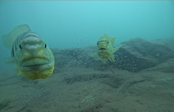
Fish might possess the flexibility to understand the place one other being’s consideration is concentrated. They usually don’t like when it’s targeted on them or on their youngsters
Male (left) and feminine (proper) emperor cichilds behaving aggressively towards a diver by flaring their gill covers.
Satoh, et al. Royal Society Open Science (CC BY 4.0)
Are you aware that uncomfortable feeling of being watched? A brand new research exhibits that fish additionally appear to know once they—or their youngsters—are being stared at, and that they don’t prefer it. The work, printed Tuesday in Royal Society Open Science,provides uncommon perception into the minds of fish.
Earlier analysis has instructed that some primates, home animals and birds appear to own what known as consideration attribution—the flexibility to understand the place one other particular person is concentrated. “It means distinguishing not simply who’s current however what that particular person is listening to,” says research creator Shun Satoh, a fish biologist at Kyoto College in Japan.
To see whether or not fish would possibly possess this potential, the workforce went to Lake Tanganyika in jap Africa to conduct totally different experiments on the emperor cichlid (Boulengerochromis microlepis), a species that’s neither too afraid of nor too aggressive towards people. Utilizing waterproof cameras, the workforce recorded how grownup fish guarding their offspring behaved when a diver checked out a fish’s eggs or its lately hatched kids, regarded in one other route, or regarded on the fish itself. The researchers additionally noticed what occurred when the diver turned 180 levels from the nest.
On supporting science journalism
Should you’re having fun with this text, take into account supporting our award-winning journalism by subscribing. By buying a subscription you’re serving to to make sure the way forward for impactful tales in regards to the discoveries and concepts shaping our world at the moment.
An evaluation of the recordings confirmed that the mother and father behaved aggressively towards the divers extra usually when the human interlopers have been staring on the offspring or the father or mother, in contrast with when the diver was trying in one other route or fully turned away.
Although the authors acknowledge the research is preliminary, the outcomes counsel that “the fish don’t reply solely to a diver’s presence but in addition to cues associated to the place the diver’s consideration is directed,” Satoh says.
The research is a superb start line to answering whether or not fish possess consideration attribution, says Gabrielle Davidson, a behavioral ecologist on the College of East Anglia in England, who was not concerned within the work. “Animals are so delicate to eyelike stimuli that we might anticipate them to seek out the gaze threatening or scary if it was directed at them,” she says. The research appears to go a step additional, nevertheless, by displaying that the fish would possibly be capable of observe the place the diver is taking a look at. “It’s not only a reflexive response to eyes being straight at them.”
Davidson thinks this potential could possibly be widespread in different fish species, however she provides that extra analysis is required to determine if the fish are literally trying on the diver’s gaze or if they’re responding to different cues.
“One of many largest challenges is to know what’s contained in the thoughts of different animals,” she says. “A lot of these additional situations and experiments can take us a step ahead to revealing the interior understanding of those animals.”
It’s Time to Stand Up for Science
Should you loved this text, I’d wish to ask in your assist. Scientific American has served as an advocate for science and business for 180 years, and proper now could be the most crucial second in that two-century historical past.
I’ve been a Scientific American subscriber since I used to be 12 years outdated, and it helped form the best way I have a look at the world. SciAm at all times educates and delights me, and evokes a way of awe for our huge, stunning universe. I hope it does that for you, too.
Should you subscribe to Scientific American, you assist make sure that our protection is centered on significant analysis and discovery; that we’ve got the assets to report on the choices that threaten labs throughout the U.S.; and that we assist each budding and dealing scientists at a time when the worth of science itself too usually goes unrecognized.
The alternating collection take a look at is a part of the usual calculus curriculum. It says that when you truncate an alternating collection, the rest is bounded by the primary time period that was omitted. This truth goes by in a blur for many college students, but it surely turns into helpful later if you want to do numerical computing.
To be extra exact, assume we’ve a collection of the shape
the place the ai are optimistic and monotonically converge to zero. Then the tail of the collection is bounded by its first time period:
The extra we will say concerning the conduct of the ai the extra we will say concerning the the rest. To date we’ve assumed that these phrases go monotonically to zero. If their variations
additionally go monotonically to zero, then we’ve an higher and decrease sure on the truncation error:
If the variations of the variations,
additionally converge monotonically to zero, we will get a bigger decrease sure and a smaller higher sure on the rest. Generally, if the variations as much as order ok of the ai go to zero monotonically, then the rest time period may be bounded as follows.
Supply: Mark B. Villarino. The Error in an Alternating Collection. American Mathematical Month-to-month, April 2018, pp. 360–364.
Our preliminary response to this query was ‘No’ or, extra exactly, ‘Not simply’—hurdle fashions will not be among the many chance fashions supported by bayesmh. One can write a program to compute the log chance of the double hurdle mannequin and use this program with bayesmh (within the spirit of http://www.stata.com/stata14/bayesian-evaluators/), however this will appear to be a frightening job if you’re not aware of Stata programming.
After which we realized, why not merely name churdle from the evaluator to compute the log chance? All we’d like is for churdle to guage the log chance at particular values of mannequin parameters with out performing iterations. This may be achieved by specifying churdle‘s choices from() and iterate(0).
Let’s have a look at an instance. We think about a easy hurdle mannequin utilizing a subset of the health dataset from [R] churdle:
Let’s assume for a second that we have already got an evaluator, mychurdle1, that returns the corresponding log-likelihood worth. We are able to match a Bayesian hurdle mannequin utilizing bayesmh as follows:
. gen byte hours0 = (hours==0) //dependent variable for the choice equation
. set seed 123
. bayesmh (hours age) (hours0 commute),
        llevaluator(mychurdle1, parameters({lnsig}))
        prior({hours:} {hours0:} {lnsig}, flat)
        saving(sim, exchange) dots

(output omitted)
We use a two-equation specification to suit this mannequin. The primary regression is specified first, and the choice regression is specified subsequent. The extra parameter, log of the usual deviation related to the primary regression, is laid out in llevaluator()‘s suboption parameters(). All parameters are assigned flat priors to acquire outcomes just like churdle. MCMC outcomes are saved in sim.dta.
Let’s now discuss in additional element a couple of log-likelihood evaluator. We’ll think about two evaluators: one utilizing churdle and one immediately implementing the log chance of the thought of hurdle mannequin.
Log-likelihood evaluator utilizing churdle
Right here we exhibit easy methods to write a log-likelihood evaluator that calls an current Stata estimation command, churdle in our instance, to compute the log chance.
program mychurdle1
        model 14.0
        args llf
        tempname b
        mat `b' = ($MH_b, $MH_p)
        seize churdle linear $MH_y1 $MH_y1x1 if $MH_touse, ///
                    choose($MH_y2x1) ll(0) from(`b') iterate(0)
        if _rc {
                if (_rc==1) { // deal with break key
                        exit _rc
                }
                scalar `llf' = .
        }
        else {
                scalar `llf' = e(ll)
        }
finish
The mychurdle1 program returns the log-likelihood worth computed by churdle on the present values of mannequin parameters. This program accepts one argument — a short lived scalar to comprise the log-likelihood worth llf. We saved present values of mannequin parameters (regression coefficients from two equations saved in vector MH_b and the additional parameter, log standard-deviation, saved in vector MH_p) in a short lived matrix b. We specified churdle‘s choices from() and iterate(0) to guage the log chance on the present parameter values. Lastly, we saved the ensuing log-likelihood worth in llf (or lacking worth if the command failed to guage the log chance).
Right here we exhibit easy methods to write a log-likelihood evaluator that computes the chance of the fitted hurdle mannequin immediately reasonably than calling churdle.
program mychurdle2
        model 14.0
        args lnf xb xg lnsig
        tempname sig
        scalar `sig' = exp(`lnsig')
        tempvar lnfj
        qui gen double `lnfj' = regular(`xg')  if $MH_touse
        qui exchange `lnfj'    = log(1 - `lnfj') if $MH_y1 <= 0 & $MH_touse
        qui exchange `lnfj'    = log(`lnfj') - log(regular(`xb'/`sig'))   ///
                              + log(normalden($MH_y1,`xb',`sig'))       ///
                                if $MH_y1 > 0 & $MH_touse
        summarize `lnfj' if $MH_touse, meanonly
        if r(N) < $MH_n {
            scalar `lnf' = .
            exit
        }
        scalar `lnf' = r(sum)
finish
The mychurdle2 program accepts 4 arguments: a short lived scalar to comprise the log-likelihood worth llf, momentary variables xb and xg containing linear predictors from the corresponding fundamental and choice equations evaluated on the present values of mannequin parameters, and momentary scalar lnsig containing the present worth of the log standard-deviation parameter. We compute and retailer the observation-level log chance in a short lived variable lnfj. World MH_y1 comprises the identify of the dependent variable from the primary (fundamental) equation, and international MH_touse marks the estimation pattern. If all observation-specific log chance contributions are nonmissing, we retailer the general log-likelihood worth in lnf or we in any other case retailer lacking.
We match our mannequin utilizing the identical syntax as earlier, besides we use mychurdle2 as this system evaluator.
We receive the identical outcomes as these obtained utilizing method 1, and we receive them a lot quicker.
Last remarks
Strategy 1 may be very easy. It may be utilized to any Stata command that returns the log chance and lets you specify parameter values at which this log chance have to be evaluated. With out an excessive amount of programming effort, you should utilize virtually any current Stata most chance estimation command with bayesmh. A drawback of method 1 is slower execution in contrast with programming the chance immediately, as in method 2. For instance, the command utilizing the mychurdle1 evaluator from method 1 took about 25 minutes to run, whereas the command utilizing the mychurdle2 evaluator from method 2 took solely 20 seconds.
Tokenization in video fashions, usually by patchification, generates an extreme and redundant variety of tokens. This severely limits video effectivity and scalability. Whereas current trajectory-based tokenizers supply a promising resolution by decoupling video period from token depend, they depend on advanced exterior segmentation and monitoring pipelines which are gradual and task-agnostic. We suggest TrajTok, an end-to-end video tokenizer module that’s totally built-in and co-trained with video fashions for a downstream goal, dynamically adapting its token granularity to semantic complexity, unbiased of video period. TrajTok incorporates a unified segmenter that performs implicit clustering over pixels in each area and time to straight produce object trajectories in a single ahead go. By prioritizing downstream adaptability over pixel-perfect segmentation constancy, TrajTok is light-weight and environment friendly, but empirically improves video understanding efficiency. With TrajTok, we implement a video CLIP mannequin skilled from scratch (TrajViT2). It achieves one of the best accuracy at scale throughout each classification and retrieval benchmarks, whereas sustaining effectivity corresponding to one of the best token-merging strategies. TrajTok additionally proves to be a flexible element past its position as a tokenizer. We present that it may be seamlessly built-in as both a probing head for pretrained visible options (TrajAdapter) or an alignment connector in vision-language fashions (TrajVLM) with particularly robust efficiency in long-video reasoning.
† College of Washington
‡ Allen Institute for Synthetic Intelligence (AI2)
Java’s revived Detroit undertaking, to allow joint utilization of Java with Python or JavaScript, is slated to quickly grow to be an official undertaking throughout the OpenJDK group.
Oracle officers plan to spotlight Detroit’s standing at JavaOne on March 17. “The principle profit [of Detroit] is it permits you to mix industry-leading Java and JavaScript or Java and Python for locations the place you need to have the ability to use each of these applied sciences collectively,” mentioned Oracle’s Georges Saab, senior vp of the Java Platform Group, in a briefing on March 12. The objective of the undertaking is to supply implementations of the javax.script API for JavaScript primarily based on the Chrome V8 JavaScript engine and for Python primarily based on CPython, in line with the Detroit undertaking web page on openjdk.org.
Initially proposed within the 2018 timeframe as a mechanism for JavaScript for use as an extension language for Java, the undertaking later fizzled when dropping sponsorship. However curiosity in it lately has been revived. The plan is to deal with Java ecosystem necessities to name different languages, with scripting for enterprise logic and quick access to AI libraries in different languages. Whereas the plan initially requires Java and Python help, different languages are slated to be added over time. The Java FFM (International Perform & Reminiscence) API is anticipated to be leveraged within the undertaking. Different objectives of the undertaking embrace:


 Structure")
 = text{softmax}left(dfrac{QK^T}{sqrt{d_k}}right)V") ,
, are question, key, and worth matrices for sequence size
  . In autoregressive technology (producing one token at a time), we can’t recompute consideration over all earlier tokens from scratch at every step — that will be
 ") computation per token generated.
computation per token generated. , we solely compute
  (the question for the brand new token), then compute consideration utilizing
  . This reduces computation from
 ") per generated token — a dramatic speedup.
per generated token — a dramatic speedup. layers,
  consideration heads, and head dimension
  , the KV cache requires:
") .
. .
. -dimensional representations. We will compress them right into a lower-dimensional latent area for storage, then decompress when wanted for computation.
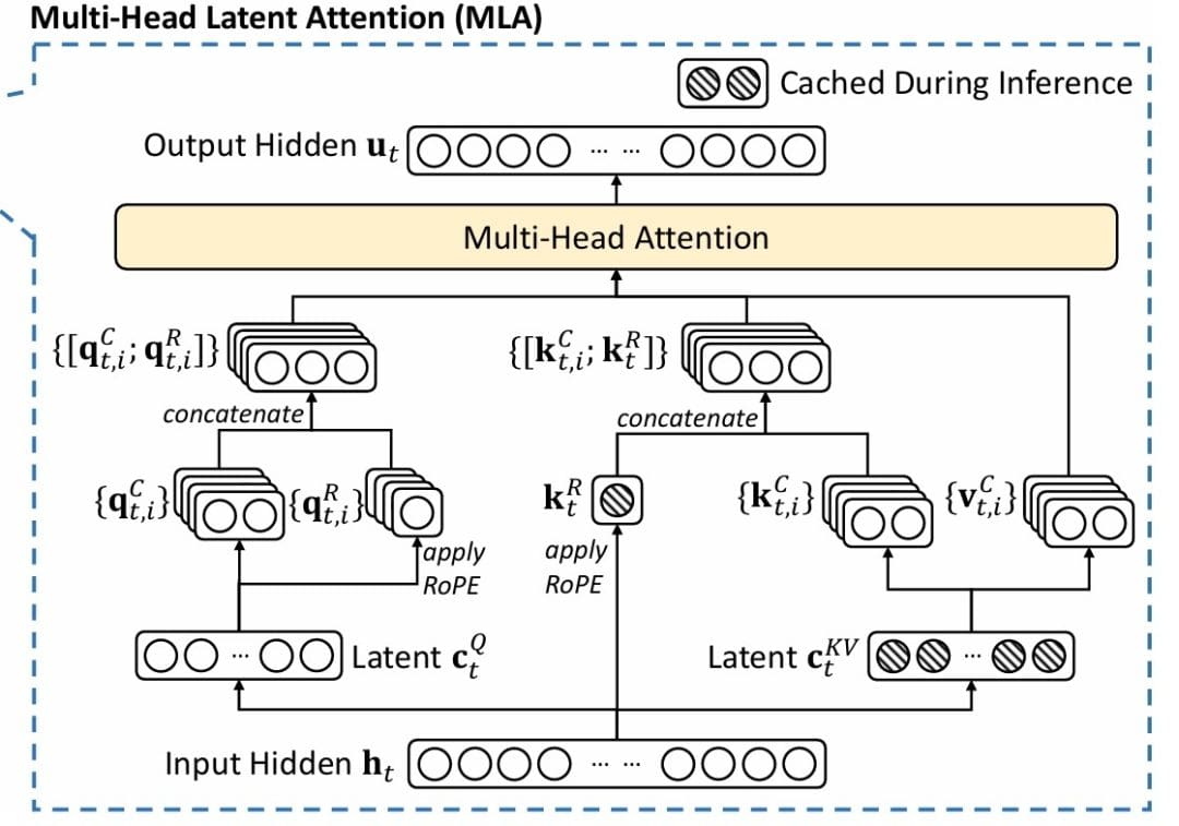
 instantly, we undertaking them by means of a low-rank bottleneck:
 in mathbb{R}^{T times r_{kv}}") ,
, is the enter,
  is the down-projection, and
  is the low-rank dimension. We solely cache
  relatively than the complete
  and
and  .
.
 ,
, are up-projection matrices. This decomposition approximates the complete key and worth matrices by means of a low-rank factorization:
  and
and  .
. , we cache
  . The discount issue is
  . For our configuration with
  and
and  , it is a 4× discount. For bigger fashions with
  and
and  , it’s a 16× discount — transformative for deployment.
 ,
, may be totally different from
  . In our configuration,
  versus
 ![Q = [Q_text{content} parallel Q_text{rope}]](https://b2633864.smushcdn.com/2633864/wp-content/latex/bb6/bb6ab893acac0d32c66ea670c4da0ab3-ffffff-000000-0.png?lossy=2&strip=1&webp=1 "Q = [Q_text{content} parallel Q_text{rope}]")
![K = [K_text{content} parallel K_text{rope}]](https://b2633864.smushcdn.com/2633864/wp-content/latex/78a/78a6aefa47951fcb5f56191065b985b4-ffffff-000000-0.png?lossy=2&strip=1&webp=1 "K = [K_text{content} parallel K_text{rope}]") ,
, denotes concatenation. The content material parts come from the compression-decompression course of described above. The positional parts are separate projections that we apply RoPE to:
")
") ,
, denotes making use of rotary embedding at place
  . This separation is essential: content material and place are independently represented and mixed solely within the consideration scores.
![Q = [Q_text{content} parallel Q_text{rope}] = [C_q W_Q parallel text{RoPE}(C_q W_{Q_text{rope}})]](https://b2633864.smushcdn.com/2633864/wp-content/latex/ba6/ba69f565f2185af859563e3059da9e47-ffffff-000000-0.png?lossy=2&strip=1&webp=1 "Q = [Q_text{content} parallel Q_text{rope}] = [C_q W_Q parallel text{RoPE}(C_q W_{Q_text{rope}})]")
![K = [K_text{content} parallel K_text{rope}] = [C_{kv} W_K parallel text{RoPE}(X W_{K_text{rope}})]](https://b2633864.smushcdn.com/2633864/wp-content/latex/df8/df82e0d3c9e02692d9042e92a9d4cc79-ffffff-000000-0.png?lossy=2&strip=1&webp=1 "K = [K_text{content} parallel K_text{rope}] = [C_{kv} W_K parallel text{RoPE}(X W_{K_text{rope}})]")
 .
.") ,
, are per-head projections. The eye scores
  naturally incorporate each content material similarity (by means of
  ) and positional info (by means of
  ).
). .
. can solely attend to positions
  , sustaining the autoregressive property.
 in mathbb{R}^{T times T}") ,
, is the efficient key dimension (content material plus RoPE dimensions). We apply consideration to values:
 ,
, is the output projection. Lastly, dropout is utilized for regularization, and the result’s added to the residual connection.
 . We retailer compression ranks (
 dimensions. Be aware that we use
  , whereas
 ![[B, T, 128]](https://b2633864.smushcdn.com/2633864/wp-content/latex/adc/adc7537e80565e8e66aadd0c2e4d8d9b-ffffff-000000-0.png?lossy=2&strip=1&webp=1 "[B, T, 128]") versus the unique
versus the unique ![[B, T, 256]](https://b2633864.smushcdn.com/2633864/wp-content/latex/164/164ef205ce8f83b5b35003a75459d10b-ffffff-000000-0.png?lossy=2&strip=1&webp=1 "[B, T, 256]") — we’ve already halved the reminiscence footprint.
— we’ve already halved the reminiscence footprint.![[B, T, H times d_text{head}]](https://b2633864.smushcdn.com/2633864/wp-content/latex/0c4/0c4a6bc039a37a204979e51949c8d0bf-ffffff-000000-0.png?lossy=2&strip=1&webp=1 "[B, T, H times d_text{head}]") to
to ![[B, H, T, d_text{head}]](https://b2633864.smushcdn.com/2633864/wp-content/latex/ca2/ca2c0152d1bb4eac8662d1600c713cc0-ffffff-000000-0.png?lossy=2&strip=1&webp=1 "[B, H, T, d_text{head}]") , shifting the pinnacle dimension earlier than the sequence dimension. This structure is required for multi-head consideration — every head operates independently, and we need to batch these operations. The
, shifting the pinnacle dimension earlier than the sequence dimension. This structure is required for multi-head consideration — every head operates independently, and we need to batch these operations. The ![[B, H, T, d_text{head} + d_text{rope}] = [B, 8, T, 96]](https://b2633864.smushcdn.com/2633864/wp-content/latex/d64/d64bff4c35da78fe1c1b2f1a5be71be1-ffffff-000000-0.png?lossy=2&strip=1&webp=1 "[B, H, T, d_text{head} + d_text{rope}] = [B, 8, T, 96]") . The eye scores will seize each content material similarity and relative place.
. The eye scores will seize each content material similarity and relative place. . The scaling issue is crucial for coaching stability — with out it, consideration logits would develop massive as dimensions enhance, resulting in vanishing gradients within the softmax. We apply the causal masks utilizing