margins is a robust device to acquire predictive margins, marginal predictions, and marginal results. It’s so highly effective that it may well work with any useful type of our estimated parameters by utilizing the expression() choice. I’m going to indicate you get hold of proportional modifications of an end result with respect to modifications within the covariates utilizing two totally different approaches for linear and nonlinear fashions.

Linear fashions with binary variables

After becoming a linear regression,
$$E(y|x) = a + b*x$$
we are able to estimate the proportional change of the fitted values with respect to a change in (x) (also called, semielasticity) utilizing margins, eydx(x). The formulation to estimate the semielasticity differ relying on whether or not (x) is steady or discrete. If (x) is steady,

start{equation}
{bf eydx} = frac{d({rm ln}widehat{y})}{dx}= frac{dy}{dx}* frac{1}{widehat{y}} = frac{widehat{b}}{widehat{y}}
tag{1}
finish{equation}
When (x) is discrete, intuitively, we expect the components can be

start{equation}
{bf eydx} = frac{E(widehat{y}|x = 1) – E(widehat{y} |x = 0)}{E(widehat{y}|x = 0)}tag{2}
finish{equation}

Nonetheless, this isn’t precisely what margins, eydx(x) calculates. As an alternative, margins obtains the distinction of (widehat{y}) relative to the bottom within the pure logarithm kind,

start{equation}
{bf eydx} = E{{rm ln}(widehat{y})|x = 1} – E{{rm ln}(widehat{y})|x = 0}tag{3}
finish{equation}
To see an instance, let’s match our mannequin with a steady and a binary variable.

. webuse lbw, clear
(Hosmer & Lemeshow knowledge)

. quietly regress bwt age i.ui

. margins, eydx(age ui)

Common marginal results                                   Variety of obs = 189
Mannequin VCE: OLS

Expression: Linear prediction, predict()
ey/dx wrt:  age 1.ui

------------------------------------------------------------------------------
             |            Delta-method
             |      ey/dx   std. err.      t    P>|t|     [95% conf. interval]
-------------+----------------------------------------------------------------
         age |    .003225    .003309     0.97   0.331     -.003303    .0097531
        1.ui |  -.2082485   .0570519    -3.65   0.000    -.3208005   -.0956964
------------------------------------------------------------------------------
Notice: ey/dx for issue ranges is the discrete change from the bottom degree.

. generate propage = _b[age]/(_b[_cons] + _b[age]*age + _b[1.ui]*ui)

. summarize propage

    Variable |        Obs        Imply    Std. dev.       Min        Max
-------------+---------------------------------------------------------
     propage |        189     .003225    .0002682   .0029186   .0039631

Let’s transfer on to ui, the proportional change of bwt with respect to a change in ui, based mostly on (2),
$$frac{widehat{{bf bwt}}|({bf ui} = 1)-widehat{{bf bwt}}|({bf ui} = 0)}{widehat{{bf bwt}}|({bf ui} = 0)}$$

. protect

. exchange ui = 0
(28 actual modifications made)

. predict bwthat0
(choice xb assumed; fitted values)

. exchange ui = 1
(189 actual modifications made)

. predict bwthat1
(choice xb assumed; fitted values)

. generate propui = (bwthat1 - bwthat0)/bwthat0

. summarize propui

    Variable |        Obs        Imply    Std. dev.       Min        Max
-------------+---------------------------------------------------------
      propui |        189    -.187989    .0030706  -.1935099  -.1760018

This time, (-0.187989) doesn’t match the semielasticity reported by margins, (-0.2082485). As we already know, margins, eydx() doesn’t calculate the proportional change with respect to a change within the categorical variable utilizing (2). As an alternative, margins, eydx() replaces the by-product on the right-hand aspect of (1) with a change from the bottom degree of the log of (y) [see (3)]. Let’s confirm this in our instance:

. generate lnbwt0  = ln(bwthat0)

. generate lnbwt1  = ln(bwthat1)

. generate propui2 = lnbwt1 - lnbwt0

. summarize propui2

    Variable |        Obs        Imply    Std. dev.       Min        Max
-------------+---------------------------------------------------------
     propui2 |        189   -.2082484    .0037771  -.2150636  -.1935868

. restore

margins, eydx() makes use of a technique based mostly on logs as a result of this methodology has higher numerical properties. As well as, if we’ve got a mannequin with the pure log of (y) on the left-hand aspect, then expressing the by-product with respect to the explicit variable because the distinction from a base class is a typical means of computing the proportional change. Suppose we’ve got a mannequin:
$$E{{rm ln}(y)} = a + b*x$$
If variable x is categorical, then (E({rm ln}(y)|x = 1) – E({rm ln}(y)|x = 0) = b). There are instances when computing (dy/dx*(1/y)) differs from the change within the logs. That is true as we transfer away from fashions which have a logarithmic illustration however even in these instances the approximation could also be enough if the proportional change within the end result given a change within the covariate is small.

If we wish to get hold of the proportional change in (2) and its related customary error, we are able to do that with margins, expression().

. margins, expression(_b[1.ui]/(_b[_cons] + _b[age]*age))
warning: choice expression() doesn't comprise choice predict() or xb().

Predictive margins                                         Variety of obs = 189
Mannequin VCE: OLS

Expression: _b[1.ui]/(_b[_cons] + _b[age]*age)

------------------------------------------------------------------------------
             |            Delta-method
             |     Margin   std. err.      z    P>|z|     [95% conf. interval]
-------------+----------------------------------------------------------------
       _cons |   -.187989   .0463242    -4.06   0.000    -.2787827   -.0971952
------------------------------------------------------------------------------

Within the expression() choice, the denominator is the expected bwt when ui = 0, and the numerator is the distinction between the prediction of bwt when ui is 1 and when ui is 0. Within the output of margins, the argument of expression() is specified after Expression:. The warning message cautions about the usage of expression() with out the predict() or xb() choice. It’s secure to disregard this message right here. We are going to see examples demonstrating the usage of these choices within the Shortcuts in expression() choice part.

Linear fashions with categorical variables

ui is a binary variable with values of 0 or 1. What if we’ve got categorical variables with greater than two teams? How can we use margins, expression() to compute a proportional change on this case? We wish to get hold of the proportional change within the predicted end result when the explicit variable modifications from the bottom degree to one among the opposite ranges. Now, I’m going to introduce the racial class variable (race =1 [White] 2 [Black] 3 [Other]) within the mannequin, as an alternative of uterine irritability.

. quietly regress bwt age i.race

. generate double propblack = _b[2.race]/(_b[_cons] + _b[age]*age)

. generate double propother = _b[3.race]/(_b[_cons] + _b[age]*age)

. summarize propblack propother

    Variable |        Obs        Imply    Std. dev.       Min        Max
-------------+---------------------------------------------------------
   propblack |        189   -.1183368    .0012359  -.1205344  -.1134239
   propother |        189   -.0927893    .0009691  -.0945124  -.0889371

. margins, expression((_b[2.race]*2.race + _b[3.race]*3.race)/       
>                     (_b[_cons]+_b[age]*age)) dydx(race)
warning: choice expression() doesn't comprise choice predict() or xb().

Common marginal results                                   Variety of obs = 189
Mannequin VCE: OLS

Expression: (_b[2.race]*2.race + _b[3.race]*3.race)/ (_b[_cons]+_b[age]*age)
dy/dx wrt:  2.race 3.race

------------------------------------------------------------------------------
             |            Delta-method
             |      dy/dx   std. err.      z    P>|z|     [95% conf. interval]
-------------+----------------------------------------------------------------
        race |
      Black  |  -.1183368    .050575    -2.34   0.019    -.2174619   -.0192117
      Different  |  -.0927893   .0358962    -2.58   0.010    -.1631447    -.022434
------------------------------------------------------------------------------
Notice: dy/dx for issue ranges is the discrete change from the bottom degree.

The handbook calculations propblack and propother match what margins reported. Right here I specified each the expression() and dydx() choices. Within the expression() choice, the numerator consists of the coefficient for every degree of race (akin to _b[2.race]) occasions the indicator for the statement belonging to the corresponding race (akin to 2.race). The coefficient represents the distinction between this race and the bottom class for race. After taking the by-product utilizing dydx() with respect to every degree,

[
frac{d({bf expression})}{d({bf 2.race})} = frac{d{({bf _b[2.race]*2.race} + {bf _b[3.race]*3.race})/({bf _b[_cons]} + {bf _b[age]*age})}}{d({bf 2.race})}
frac{d({bf expression})}{d({bf 3.race})} = frac{d{({bf _b[2.race]*2.race} + {bf _b[3.race]*3.race})/({bf _b[_cons]} + {bf _b[age]*age})}}{d({bf 3.race})}
]

we find yourself with the expressions of proportional modifications with respect to Black and Different moms,
$$
{bf _b[2.race]}/({bf _b[_cons]} + {bf _b[age]*age})
{bf _b[3.race]}/({bf _b[_cons]} + {bf _b[age]*age})
$$
We might have as an alternative used two separate margins, expression() instructions to compute the proportional change for every group in contrast with the bottom, much like what we did beforehand for the binary variable. Placing them in a single expression makes it doable to additional manipulate these margins. As an illustration, by estimating each proportional modifications with one margins command, we now get hold of each estimates together with the covariance of the estimates, and this enables us to check for a distinction within the proportional modifications.

Nonlinear fashions

The computations will be generalized to nonlinear fashions; the key distinction can be the hyperlink perform to compute the expected end result. Within the subsequent instance, we use probit and Poisson regressions.

. quietly probit low age i.race

. margins, expression((regular(_b[_cons] + _b[age]*age        
>                   + _b[2.race]*2.race + _b[3.race]*3.race) 
>                   - regular(_b[_cons] + _b[age]*age))/      
>                     regular(_b[_cons] + _b[age]*age)) dydx(race)
warning: choice expression() doesn't comprise choice predict() or xb().

Common marginal results                                   Variety of obs = 189
Mannequin VCE: OIM

Expression: (regular(_b[_cons] + _b[age]*age + _b[2.race]*2.race +
            _b[3.race]*3.race) - regular(_b[_cons] + _b[age]*age))/
            regular(_b[_cons] + _b[age]*age)
dy/dx wrt:  2.race 3.race

------------------------------------------------------------------------------
             |            Delta-method
             |      dy/dx   std. err.      z    P>|z|     [95% conf. interval]
-------------+----------------------------------------------------------------
        race |
      Black  |    .662603   .5016623     1.32   0.187    -.3206371    1.645843
      Different  |   .4874649   .3652971     1.33   0.182    -.2285042    1.203434
------------------------------------------------------------------------------
Notice: dy/dx for issue ranges is the discrete change from the bottom degree.

Within the probit regression, we modeled the likelihood of getting a low-birthweight child by utilizing moms’ age and racial classes. We obtained the proportional modifications of predicted likelihood evaluating Black with White moms and Different with White moms.

. webuse dollhill3, clear
(Doll and Hill (1966))

. quietly poisson deaths smokes i.agecat, publicity(pyears)

.  margins, expression((exp(_b[smokes]*smokes + _b[2.agecat]*2.agecat       
>                    + _b[3.agecat]*3.agecat + _b[4.agecat]*4.agecat       
>                    + _b[5.agecat]*5.agecat + _ b[_cons])*pyears          
>                     - exp(_b[smokes]*smokes + _ b[_cons])*pyears)/       
>                      (exp(_b[smokes]*smokes + _ b[_cons])*pyears))       
>                       dydx(agecat)
warning: choice expression() doesn't comprise choice predict() or xb().

Common marginal results                                    Variety of obs = 10
Mannequin VCE: OIM

Expression: (exp(_b[smokes]*smokes + _b[2.agecat]*2.agecat +
            _b[3.agecat]*3.agecat + _b[4.agecat]*4.agecat +
            _b[5.agecat]*5.agecat + _ b[_cons])*pyears -
            exp(_b[smokes]*smokes + _ b[_cons])*pyears)/
            (exp(_b[smokes]*smokes + _ b[_cons])*pyears)
dy/dx wrt:  2.agecat 3.agecat 4.agecat 5.agecat

------------------------------------------------------------------------------
             |            Delta-method
             |      dy/dx   std. err.      z    P>|z|     [95% conf. interval]
-------------+----------------------------------------------------------------
      agecat |
      45–54  |   3.410584   .8605197     3.96   0.000     1.723996    5.097171
      55–64  |    12.8392   2.542638     5.05   0.000      7.85572    17.82268
      65–74  |   27.51678   5.269878     5.22   0.000     17.18801    37.84555
      75–84  |   39.45121   7.775511     5.07   0.000     24.21148    54.69093
------------------------------------------------------------------------------
Notice: dy/dx for issue ranges is the discrete change from the bottom degree.

Within the Poisson regression, the variety of deaths was defined by smoking standing and age class. The proportional modifications of predicted variety of deaths have been computed by evaluating every age group with the bottom.

margins operates on marginal prediction of the end result, the place the prediction equals xb in linear regression, equals ({rm regular}(xb)) in probit regression, and equals ({rm exp}(xb) occasions {rm publicity}) in Poisson regression. Moreover, margins computes the prediction for every statement and stories the imply because the predictive margins.

Shortcuts within the expression() choice

The useful types we feed into margins, expression() will be as versatile and sophisticated as wanted. There are a number of shortcuts that I wish to spotlight right here. Let’s return to the probit regression.

. quietly probit low c.age##i.race

. margins, eydx(age)

Common marginal results                                   Variety of obs = 189
Mannequin VCE: OIM

Expression: Pr(low), predict()
ey/dx wrt:  age

------------------------------------------------------------------------------
             |            Delta-method
             |      ey/dx   std. err.      z    P>|z|     [95% conf. interval]
-------------+----------------------------------------------------------------
         age |  -.0318742   .0234627    -1.36   0.174    -.0778603    .0141118
------------------------------------------------------------------------------

I launched a two-way, full-factorial time period between age and race. Right here is the useful kind spelled out to acquire margins, eydx(age):

[
{bf xb} = {bf _b[age]*age} + {bf _b[2.race#c.age]*2.race*age} +{bf _b[3.race#c.age]*3.race*age}
+ {bf _b[2.race]*2.race} + {bf _b[3.race]*3.race} + {bf _b[_cons]} [.1in]
frac{d {rm ln}{{rm regular}(xb)}}{d {bf age}} =frac{{bf _b[age]} + {bf _b[2.race#c.age]*2.race} + {bf _b[3.race#c.age]*3.race}}{{rm regular}(xb)} occasions {rm normalden}(xb)
]

Within the expression() choice, it isn’t mandatory to jot down out the expression for issues like linear prediction; thus, the above proportional change will be computed by

. margins, expression((_b[age] + _b[2.race#c.age]*2.race 
>     + _b[3.race#c.age]*3.race)*normalden(predict(xb))/regular(predict(xb)
> ))

Predictive margins                                         Variety of obs = 189
Mannequin VCE: OIM

Expression: (_b[age] + _b[2.race#c.age]*2.race +
            _b[3.race#c.age]*3.race)*normalden(predict(xb))/
            > regular(predict(xb))

------------------------------------------------------------------------------
             |            Delta-method
             |     Margin   std. err.      z    P>|z|     [95% conf. interval]
-------------+----------------------------------------------------------------
       _cons |  -.0318742   .0234627    -1.36   0.174    -.0778603    .0141118
------------------------------------------------------------------------------

the place predict(xb) is a shortcut to discuss with the linear prediction. Additional, regular(predict(xb)) will be changed with predict(pr), the place pr stands for likelihood of the optimistic end result. The expression() choice in margins lets us assemble any capabilities of the estimated parameters and feed them again to margins. We then can use all of the computations and graphical instruments with marginsplot to visualise the consequence.

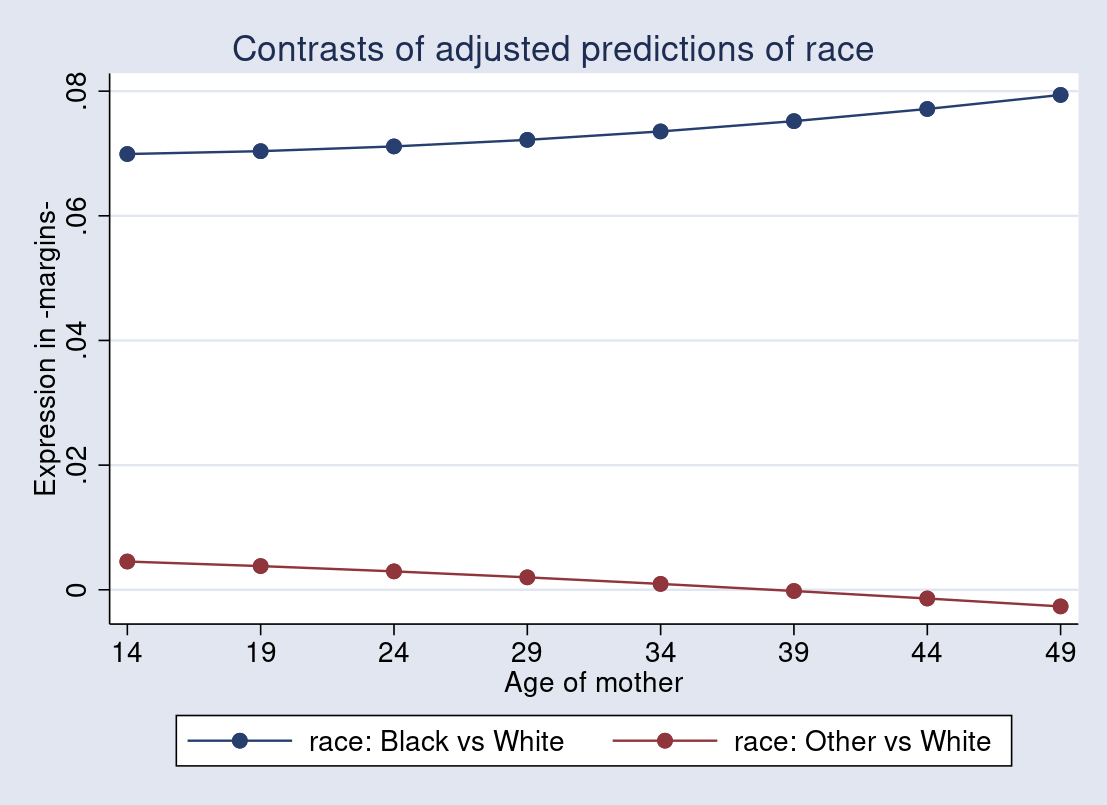
. quietly margins r.race, expression((_b[age] + _b[2.race#c.age]*2.race     
>    + _b[3.race#c.age]*3.race)*normalden(predict(xb))/regular(predict(xb))) 
>          at(age=(14(5)50))

. quietly marginsplot, noci ytitle("expression in -margins-")

I obtained the proportional modifications of predicted likelihood of getting a low-birthweight child with respect to the modifications in moms’ ages by evaluating these from Black moms and Different moms with these from White moms. The distinction can also be visualized throughout a variety of moms’ ages from 14 by way of 50. The marginally diverging sample may point out the interplay impact that racial class moderates the connection between the likelihood of getting a low-birthweight child and moms’ age.

Conclusion
On this put up, we realized use the expression() choice with the margins command to acquire proportional modifications of the end result with respect to the modifications in categorical covariates in each linear and nonlinear fashions. The expression() choice is a flexible and highly effective choice that enables any useful type of estimated parameters and lets margins function on the prediction of the end result.