Final Monday, the identical day it introduced itself to the world in Wired, R3 despatched us a sweeping disavowal of our findings. It stated Schloendorn “by no means made any assertion relating to hypothetical ‘non-sentient human clones’ [that] can be carried by surrogates.” Probably the most overarching of those challenges was its insistence that “any allegations of intent or conspiracy to create human clones or people with mind injury are categorically false.”
However even Schloendorn and his cofounder, Alice Gilman, can’t appear to stay away from the subject. Simply final September, the pair offered at Abundance Longevity, a $70,000-per-ticket occasion in Boston organized by the anti-aging promoter Peter Diamandis. Though the presentation to about 40 individuals was not recorded and was meant to be confidential, a duplicate of the agenda for the occasion exhibits that Schloendorn was there to stipulate his “closing bid to defeat growing older” in a session referred to as “Full Physique Alternative.”
In response to an individual who was there, each animal analysis and private clones for spare organs have been mentioned. Through the presentation, Gilman and Schloendorn even stood in entrance of a picture of a cloning needle. Pressed on whether or not this was a speak about brainless clones, Gilman instructed us that whereas R3’s present enterprise is changing animal fashions, “the staff reserves the fitting to carry hypothetical futuristic discussions.”
MIT Know-how Evaluation discovered no proof that R3 has cloned anybody, and even any animal larger than a rodent. What we did discover have been paperwork, extra assembly agendas, and different sources outlining a technical highway map for what R3 referred to as “physique alternative cloning” in a 2023 letter to supporters. That highway map concerned enhancements to the cloning course of and genetic wiring diagrams for easy methods to create animals with out full brains.
A baby with hydranencephaly, a uncommon situation by which many of the mind is lacking. Might a human clone even be created with out a lot of a mind as an moral supply of spare organs?
DIMITRI AGAMANOLIS, M.D. VIA WIKIPEDIA
A most important function of the fundraising, traders say, was to help efforts to attempt these strategies in monkeys from a base within the Caribbean. That supplied a path to a nearer-term marketing strategy for extra moral medical experiments and toxicology testing—if the corporate may develop what it now calls monkey “organ sacks.” Nonetheless, this work would clearly inform any doable human model.
Although he holds a PhD, Schloendorn is a biotech outsider who has revealed little and is greatest recognized for having as soon as outfitted a DIY lab in his Bay Space storage. Nonetheless, his ties to the experimental fringe of longevity science have earned him a community in Silicon Valley and allies at a risk-taking US well being innovation company, ARPA-H. Collectively together with his success at elevating cash from traders, this alerts that the brainless-clone idea needs to be taken severely by a wider group of scientists, docs, and ethicists, a few of whom expressed grave considerations.
“It sounds loopy, in my view,” stated Jose Cibelli, a researcher at Michigan State College, after MIT Know-how Evaluation described R3’s brainless-clone concept to him. “How do you show security? What’s security if you’re attempting to create an irregular human?”
Twenty-five years in the past, Cibelli was among the many first scientists to attempt to clone human embryos, however he was attempting to acquire matched stem cells, not make a child. “There is no such thing as a restrict to human creativeness and methods to earn cash, however there need to be boundaries,” he says. “And that is the boundary of creating a human being who shouldn’t be a human being.”
Breakthroughs, discoveries, and DIY ideas despatched six days per week.
We by no means absolutely misplaced our love for bodily media. Tangible copies of music, motion pictures, and books have by no means been fully out of date. In truth, accumulating has come again in vogue amongst youthful generations. That stated, bodily media isn’t without end. It may rot, put on, and disintegrate in methods cloud storage can’t.
The reality is, many people aren’t precisely certain how lengthy our digital media storage lasts, or what components may have an effect on that longevity. Correct knowledge storage is essential for managing info and defending it from loss. However it’s not nearly security; Information storage additionally entails organizing knowledge to make it accessible and helpful.
There are a number of sorts of digital storage gadgets obtainable. The most typical ones are laborious disk drives (HDDs), stable state drives (SSDs), common serial bus (USB) flash drives, reminiscence playing cards, and network-attached storage (NAS) gadgets. Every sort has its personal benefits and particular use circumstances. For instance, a HDD makes use of spinning disks and magnetic heads to learn and write knowledge, they usually’re generally utilized in desktop and laptop computer computer systems for storing working programs, functions, and private information. HDDs usually supply massive storage capacities at comparatively decrease prices in comparison with different storage gadgets.
Not like HDDs, SSDs use flash reminiscence know-how to retailer knowledge electronically. SSDs don’t have any shifting components, making them sooner, extra dependable, and quieter than HDDs. They’re generally used to reinforce the efficiency of laptops and desktops, high-performance servers and gaming consoles.
Lastly, NAS is a storage gadget that connects to your community and offers a centralized storage choice for a number of gadgets. It’s like a devoted file server that lets you retailer and entry information from completely different gadgets, akin to computer systems, smartphones, and tablets. It’s based mostly on the identical SSD or HDD tech outlined above, nevertheless it’s accessed otherwise.
So how lengthy are you able to fairly depend on them? Right here’s some steering…
HARD DISK DRIVES (HDDs)
Most HDDs final three to 5 years earlier than parts begin to fail. Nevertheless, some element failure doesn’t essentially imply your knowledge is irrecoverably misplaced. As with all media storing important knowledge, investing in higher-quality drives can even make a distinction. In the event you hear your drive beginning to make uncommon noises or vibrate greater than it usually does, it might be time to interchange it. Even when it’s seemingly working positive, drives can fail with no warning so make sure that to maintain a second copy someplace.
SOLID STATE DRIVES (SSDs)
SSDs are constructed for longevity and usually outlive many different parts in your pc. With regular day-to-day utilization, most SSDs will final anyplace from 5 to 10 years, and doubtlessly longer. For the common house consumer writing 20-40GB of knowledge per day, an SSD can supply many years of dependable efficiency. However you do must think about environmental circumstances – excessive temperatures can have an effect on efficiency and lifespan – drive high quality and quantity of “typical” utilization.
NETWORK-ATTACHED STORAGE (NAS)
On common, an NAS drive is designed to final round three to 5 years. However like HDDs and SDDS, this will change based mostly on the standard of the drive, utilization patterns, environmental circumstances, and upkeep practices. NAS programs usually use multi-drive enclosures that generally enable customers to simply swap drives at common intervals. Whereas this will add helpful redundancy, it additionally introduces extra parts to fail.
Increased-quality drives are inclined to have higher parts and are constructed to face up to extra rigorous utilization. Drives which are continuously accessed and subjected to heavy learn/write operations might put on out sooner in comparison with drives that have lighter utilization. Environmental circumstances, akin to temperature and humidity, can impression the lifespan of a NAS drive. Extreme warmth and moisture may cause parts to degrade sooner.
USB FLASH DRIVE
The benefit of flash drives is that they’re transportable, sturdy, and have massive storage capability (as much as 4TB). They’re additionally capable of retain the reminiscence even after the ability is turned off. In the event you merely write knowledge to a USB flash drive and put it away in a cool, dry place, it may well final greater than 10 years. Clearly, fixed use will have an effect on that lifespan.
MEMORY CARDS
In accordance with SD card requirements, a reminiscence cell ought to be capable to protect knowledge for not less than ten years if stored at a constant temperature. The standard of the cardboard itself, the depth of use, and the environmental circumstances can all affect the precise lifespan of the SD playing cards. Like the opposite choices, frequent writing and deleting of knowledge, excessive temperatures, and even humidity can speed up the getting older strategy of the reminiscence cells.
The interface can usually be the failure level for a reminiscence card. An SD card, for instance, has plastic enamel that may break over repeated makes use of. In that occasion, your knowledge will likely be safely saved, however you received’t be capable to entry it. In the event you hear an SD card creaking or making any noise as you insert it into your gadget, it’s probably time for a brand new one.
Richard Feynman mentioned that nearly all the things turns into fascinating for those who look into it deeply sufficient. Wanting up numbers in a desk is actually not fascinating, nevertheless it turns into extra fascinating while you dig into how properly you’ll be able to fill within the gaps.
If you wish to know the worth of a tabulated operate between values of x given within the desk, it’s important to use interpolation. Linear interpolation is commonly satisfactory, however you may get extra correct outcomes utilizing higher-order interpolation.
Suppose you might have a operate f(x) tabulated at x = 3.00, 3.01, 3.02, …, 3.99, 4.00 and also you wish to approximate the worth of the operate at π. You would approximate f(π) utilizing the values of f(3.14) and f(3.15) with linear interpolation, however you may additionally reap the benefits of extra factors within the desk. For instance, you may use cubic interpolation to calculate f(π) utilizing f(3.13), f(3.14), f(3.15), and f(3.16). Or you may use twenty ninth diploma interpolation with the values of f at 3.00, 3.01, 3.02, …, 3.29.
The Lagrange interpolation theorem permits you to compute an higher certain in your interpolation error. Nevertheless, the theory assumes the values at every of the tabulated factors are actual. And for bizarre use, you’ll be able to assume the tabulated values are actual. The most important supply of error is often the dimensions of the hole between tabulated x values, not the precision of the tabulated values. Tables have been designed so that is true [1].
The certain on order n interpolation error has the shape
c hn + 1 + λ δ
the place h is the spacing between interpolation factors and δ is the error within the tabulated values. The worth of c depends upon the derivatives of the operate you’re interpolating [2]. The worth of λ is at the very least 1 since λδ is the “interpolation” error on the tabulated factors.
The accuracy of an interpolated worth can’t be higher than δ typically, and so that you decide the worth of n that makes c hn + 1 lower than δ. Any increased worth of n isn’t useful. And actually increased values of n are dangerous since λ grows exponentially as a operate of n [3].
See the subsequent publish for mathematical particulars concerning the λs.
Examples
Let’s take a look at a particular instance. Right here’s a bit of a desk for pure logarithms from A&S.
Right here h = 10−3, and so linear interpolation would offer you an error on the order of h² = 10−6. You’re by no means going to get error lower than 10−15 since that’s the error within the tabulated values, so 4th order interpolation offers you about as a lot precision as you’re going to get. Rigorously bounding the error would require utilizing the values of c and λ above which might be particular to this context. In actual fact, the interpolation error is on the order of 10−8 utilizing fifth order interpolation, and that’s the very best you are able to do.
I’ll briefly point out a pair extra examples from A&S. The e-book features a desk of sine values, tabulated to 23 decimal locations, in increments of h = 0.001 radians. A tough estimate would recommend seventh order interpolation is as excessive as you must go, and actually the e-book signifies that seventh order interpolation gives you 9 figures of accuracy,
One other desk from A&S offers values of the Bessel operate J0 in with 15 digit values in increments of h = 0.1. It says that eleventh order interpolation gives you 4 decimal locations of precision. On this case, pretty high-order interpolation is helpful and even crucial. A lot of decimal locations are wanted within the tabulated values relative to the output precision as a result of the spacing between factors is so huge.
Associated posts
[1] I say have been due to course individuals not often lookup operate values in tables anymore. Tables and interpolation are nonetheless broadly used, simply indirectly by individuals; computer systems do the lookup and interpolation on their behalf.
[2] For capabilities like sine, the worth of c doesn’t develop with n, and actually decreases slowly as n will increase. However for different capabilities, c can develop with n, which might trigger issues like Runge phenomena.
[2] The fixed λ grows exponentially with n for evenly spaced interpolation factors, and values in a desk are evenly spaced. The fixed λ grows solely logarithmically for Chebyshev spacing, however this isn’t sensible for a normal goal desk.
Transitions of any scale are sometimes met with a mixture of pleasure and trepidation. One 12 months in the past, after we launched into the journey emigrate the Black Belt Academy to our new Studying Administration System (LMS), MindTickle, the stakes had been excessive. We weren’t simply shifting information; we had been migrating the educational legacy of over 90,000 companion people and defending 300,000 studying information.
As we speak, as we have a good time our one-year anniversary on the platform, these preliminary “migration jitters” have been changed by a story of strategic collaboration, AI-driven innovation, and a remodeled studying expertise.
A Strategic Alliance for World Attain
Our success over the previous 12 months hasn’t simply been about adopting new software program; it’s been concerning the deep, collaborative partnership we’ve constructed with the MindTickle crew. By working as strategic allies, we’ve pushed the boundaries of what a studying platform can do, specializing in key areas that add instant worth to our companions:
Multi-lingual trainings powered by Black Belt AI Translation device: To help our world ecosystem, we’ve launched automated translations, making studying supplies quickly out there in Spanish, Portuguese, French, German, Korean, Japanese, and Mandarin.
Improved Navigation: We’ve co-developed an interface that ensures discovering the proper coaching is quicker and extra intuitive, permitting companions to spend much less time looking and extra time rising.
Strong Scores & Suggestions Techniques: We’ve closed the loop between learners and content material creators. Our new suggestions techniques permit us to hearken to our companions’ wants and pivot our content material technique primarily based on their direct enter, sustaining a present CSAT score of 4.8 out of 5.
AI Validation & Gross sales Pitch Software: Now we have launched cutting-edge AI validation that gives companions with immediate, automated checks on their progress. That is additional enhanced by our AI Gross sales Pitch device, which permits companions to observe presenting their worth propositions in a secure setting and obtain useful, AI-calibrated suggestions to strengthen their real-world gross sales efficiency.
Synergy between Inner Cisco Gross sales pressure and companions. With the discharge of Quarterly Improvement Focus content material, we’re offering companions with the identical coaching materials that’s out there for Cisco inside gross sales group. Companions and Cisco groups can additional align with what our prospects want, and the way we will present worth.
Alignment and the Cisco 360 Associate Program
Black Belt Academy has grow to be a cornerstone of the brand new Cisco 360 Associate Program. By aligning our curriculum with the Associate Worth Index for every Portfolio, we be certain that our companions are studying in lockstep with Cisco’s personal strategic objectives. This synergy is driving a extra constant and sturdy development engine for our complete ecosystem.
The Outcomes: Impression by the Numbers
Probably the most rewarding a part of this primary 12 months of collaboration has been seeing the tangible enterprise outcomes:
Unprecedented Progress: In Q1 FY2026 alone, we achieved a record-breaking 105,200 new certifications—a staggering 160% year-over-year development.
Rising Experience: This quarter noticed 22,300 licensed people, a 90% improve in YoY, underscoring the increasing pool of expert professionals.
Deep Engagement: Our “needle mover” companions (these representing 80% of our enterprise) are totally on board. 95% of those important companions are energetic within the Academy, highlighting a direct correlation between studying and enterprise influence.
Trying Ahead: The Imaginative and prescient for 12 months Two
What began as a profitable migration has advanced right into a powerhouse of companion enablement. However we’re simply getting began. As we glance to the longer term, our partnership with MindTickle will give attention to creating an much more built-in and seamless expertise:
Integrating eLearning and Stay Coaching: We’re working towards a richer, “all-in-one” ecosystem that seamlessly blends on-demand modules with dwell coaching modalities, powered by AI and calibrated by actual specialists.
B2B Integration Improvement: We’re exploring methods to attach Black Belt Academy immediately with our companions’ personal Studying Administration Techniques. This is able to permit us to supply high-quality content material immediately inside their native environments—offering the proper data, the place they want it, once they want it.
As we transfer into 12 months two, our objective stays the identical: to offer a world-class, AI-calibrated studying expertise that empowers each companion to guide out there.
Thanks to our companions and the MindTickle crew for becoming a member of us on this journey. The very best is but to return!
We’d love to listen to what you assume. Ask a Query, Remark Beneath, and Keep Linked with #CiscoPartners on social!
With the abundance of nice libraries, in R, for statistical computing, why would you be fascinated by TensorFlow Likelihood (TFP, for brief)? Nicely – let’s take a look at an inventory of its parts:
Distributions and bijectors (bijectors are reversible, composable maps)
Probabilistic modeling (Edward2 and probabilistic community layers)
Probabilistic inference (through MCMC or variational inference)
Now think about all these working seamlessly with the TensorFlow framework – core, Keras, contributed modules – and likewise, working distributed and on GPU. The sphere of doable functions is huge – and much too numerous to cowl as an entire in an introductory weblog publish.
As an alternative, our goal right here is to supply a primary introduction to TFP, specializing in direct applicability to and interoperability with deep studying.
We’ll rapidly present tips on how to get began with one of many fundamental constructing blocks: distributions. Then, we’ll construct a variational autoencoder just like that in Illustration studying with MMD-VAE. This time although, we’ll make use of TFP to pattern from the prior and approximate posterior distributions.
We’ll regard this publish as a “proof on idea” for utilizing TFP with Keras – from R – and plan to observe up with extra elaborate examples from the realm of semi-supervised illustration studying.
To put in TFP along with TensorFlow, merely append tensorflow-probability to the default record of additional packages:
library(tensorflow)install_tensorflow( extra_packages =c("keras", "tensorflow-hub", "tensorflow-probability"), model ="1.12")
Now to make use of TFP, all we have to do is import it and create some helpful handles.
And right here we go, sampling from a typical regular distribution.
Now that’s good, but it surely’s 2019, we don’t wish to must create a session to judge these tensors anymore. Within the variational autoencoder instance beneath, we’re going to see how TFP and TF keen execution are the proper match, so why not begin utilizing it now.
To make use of keen execution, we’ve to execute the next traces in a contemporary (R) session:
Opposite to what it would appear to be, this isn’t a multivariate regular. As indicated by batch_shape=(3,), it is a “batch” of impartial univariate distributions. The truth that these are univariate is seen in event_shape=(): Every of them lives in one-dimensional occasion house.
If as an alternative we create a single, two-dimensional multivariate regular:
This instance defines a batch of three two-dimensional multivariate regular distributions.
Changing between batch shapes and occasion shapes
Unusual as it might sound, conditions come up the place we wish to remodel distribution shapes between these sorts – in reality, we’ll see such a case very quickly.
tfd$Impartial is used to transform dimensions in batch_shape to dimensions in event_shape.
Here’s a batch of three impartial Bernoulli distributions.
Right here reinterpreted_batch_ndims tells TFP how lots of the batch dimensions are getting used for the occasion house, beginning to rely from the appropriate of the form record.
With this fundamental understanding of TFP distributions, we’re able to see them utilized in a VAE.
We’ll take the (not so) deep convolutional structure from Illustration studying with MMD-VAE and use distributions for sampling and computing chances. Optionally, our new VAE will have the ability to study the prior distribution.
Concretely, the next exposition will include three components.
First, we current frequent code relevant to each a VAE with a static prior, and one which learns the parameters of the prior distribution.
Then, we’ve the coaching loop for the primary (static-prior) VAE. Lastly, we talk about the coaching loop and extra mannequin concerned within the second (prior-learning) VAE.
Presenting each variations one after the opposite results in code duplications, however avoids scattering complicated if-else branches all through the code.
The second VAE is accessible as a part of the Keras examples so that you don’t have to repeat out code snippets. The code additionally comprises further performance not mentioned and replicated right here, corresponding to for saving mannequin weights.
So, let’s begin with the frequent half.
On the danger of repeating ourselves, right here once more are the preparatory steps (together with a couple of further library hundreds).
Now let’s see what adjustments within the encoder and decoder fashions.
Encoder
The encoder differs from what we had with out TFP in that it doesn’t return the approximate posterior means and variances straight as tensors. As an alternative, it returns a batch of multivariate regular distributions:
# you would possibly wish to change this relying on the datasetlatent_dim<-2encoder_model<-operate(title=NULL){keras_model_custom(title =title, operate(self){self$conv1<-layer_conv_2d( filters =32, kernel_size =3, strides =2, activation ="relu")self$conv2<-layer_conv_2d( filters =64, kernel_size =3, strides =2, activation ="relu")self$flatten<-layer_flatten()self$dense<-layer_dense(items =2*latent_dim)operate(x, masks=NULL){x<-x%>%self$conv1()%>%self$conv2()%>%self$flatten()%>%self$dense()tfd$MultivariateNormalDiag( loc =x[, 1:latent_dim], scale_diag =tf$nn$softplus(x[, (latent_dim+1):(2*latent_dim)]+1e-5))}})}
We don’t learn about you, however we nonetheless benefit from the ease of inspecting values with keen execution – quite a bit.
Now, on to the decoder, which too returns a distribution as an alternative of a tensor.
Decoder
Within the decoder, we see why transformations between batch form and occasion form are helpful.
The output of self$deconv3 is four-dimensional. What we want is an on-off-probability for each pixel.
Previously, this was achieved by feeding the tensor right into a dense layer and making use of a sigmoid activation.
Right here, we use tfd$Impartial to successfully tranform the tensor right into a chance distribution over three-dimensional photos (width, top, channel(s)).
Now the loss consists of the same old ELBO parts: reconstruction loss and KL divergence.
The reconstruction loss we straight get hold of from TFP, utilizing the realized decoder distribution to evaluate the probability of the unique enter.
Aside from these adjustments resulting from utilizing TFP, the coaching course of is simply regular backprop, the best way it appears to be like utilizing keen execution.
Now let’s see how as an alternative of utilizing the usual isotropic Gaussian, we might study a mix of Gaussians.
The selection of variety of distributions right here is fairly arbitrary. Simply as with latent_dim, you would possibly wish to experiment and discover out what works finest in your dataset.
mixture_components<-16learnable_prior_model<-operate(title=NULL, latent_dim, mixture_components){keras_model_custom(title =title, operate(self){self$loc<-tf$get_variable( title ="loc", form =record(mixture_components, latent_dim), dtype =tf$float32)self$raw_scale_diag<-tf$get_variable( title ="raw_scale_diag", form =c(mixture_components, latent_dim), dtype =tf$float32)self$mixture_logits<-tf$get_variable( title ="mixture_logits", form =c(mixture_components), dtype =tf$float32)operate(x, masks=NULL){tfd$MixtureSameFamily( components_distribution =tfd$MultivariateNormalDiag( loc =self$loc, scale_diag =tf$nn$softplus(self$raw_scale_diag)), mixture_distribution =tfd$Categorical(logits =self$mixture_logits))}})}
In TFP terminology, components_distribution is the underlying distribution sort, and mixture_distribution holds the possibilities that particular person parts are chosen.
Observe how self$loc, self$raw_scale_diag and self$mixture_logits are TensorFlow Variables and thus, persistent and updatable by backprop.
And that’s it! For us, each VAEs yielded related outcomes, and we didn’t expertise nice variations from experimenting with latent dimensionality and the variety of combination distributions. However once more, we wouldn’t wish to generalize to different datasets, architectures, and many others.
Talking of outcomes, how do they give the impression of being? Right here we see letters generated after 40 epochs of coaching. On the left are random letters, on the appropriate, the same old VAE grid show of latent house.
Hopefully, we’ve succeeded in displaying that TensorFlow Likelihood, keen execution, and Keras make for a pretty mixture! In case you relate complete quantity of code required to the complexity of the duty, in addition to depth of the ideas concerned, this could seem as a fairly concise implementation.
Within the nearer future, we plan to observe up with extra concerned functions of TensorFlow Likelihood, largely from the realm of illustration studying. Keep tuned!
Clanuwat, Tarin, Mikel Bober-Irizar, Asanobu Kitamoto, Alex Lamb, Kazuaki Yamamoto, and David Ha. 2018. “Deep Studying for Classical Japanese Literature.” December 3, 2018. https://arxiv.org/abs/cs.CV/1812.01718.
The Handala hackers related to Iran have breached the non-public e-mail account of FBI Director Kash Patel and revealed photographs and paperwork.
The FBI has confirmed the compromise, saying that the stolen knowledge was not current and didn’t embrace any authorities knowledge.
On Friday, the Handala risk actor introduced on one in every of their web sites that Patel has been added to the listing of their victims, alleging that they compromised “the so-called ‘impenetrable’ techniques of the FBI” in just some hours.
Nevertheless, the hackers had breached the FBI Director’s private Gmail inbox.
“All private and confidential info of Kash Patel, together with emails, conversations, paperwork, and even categorized information, is now accessible for public obtain,” the Handala hackers mentioned earlier than publishing proof of the breach.
Handala hackers saying FBI Director Patel’s inbox hack supply: BleepingComputer
Shortly after the announcement, the risk actor revealed a set of watermarked private photographs and paperwork extracted from Patel’s inbox, together with e-mail correspondence from earlier than changing into FBI director.
In an announcement for BleepingComputer, the FBI mentioned that it was conscious of hackers “concentrating on Director Patel’s private e-mail info.”
The company additional notes that it has taken each crucial precaution to cut back any destructive impression that will outcome from this exercise.
“The FBI is conscious of malicious actors concentrating on Director Patel’s private e-mail info, and we’ve taken all crucial steps to mitigate potential dangers related to this exercise. The knowledge in query is historic in nature and entails no authorities info,” – the Federal Bureau of Investigation
The Handala hacktivist group has beforehand breached the Microsoft surroundings of medical know-how large Stryker and wiped practically 80,000 gadgets.
Also referred to as Handala Hack, Hatef, and Hamsa, the actor emerged in December 2023 and is a hacktivist persona finishing up cyber actions for Iran’s Ministry of Intelligence and Safety (MOIS).
Within the assertion on the compromise of Director Patel’s private e-mail account, the FBI reiterated the $10 million reward from the Division of State’s Rewards for Justice “for info resulting in the identification of the Handala Hack Staff out of Iran.”
Automated pentesting proves the trail exists. BAS proves whether or not your controls cease it. Most groups run one with out the opposite.
This whitepaper maps six validation surfaces, exhibits the place protection ends, and gives practitioners with three diagnostic questions for any device analysis.
One of many purported benefits of self-driving automobile tech is that each automobile can be taught from one automobile’s errors. Right here’s how Waymo places it on its web site: “The Waymo Driver learns from the collective experiences gathered throughout our fleet, together with earlier {hardware} generations.”
However in Austin, Waymo’s automobiles struggled for months to learn to cease for college buses as drivers picked up and dropped off youngsters. An official with the Austin Unbiased College District (AISD) alleged that the automobiles had, in a minimum of 19 situations, “illegally and dangerously” handed the district’s faculty buses whereas their crimson lights have been flashing and their cease arms have been prolonged reasonably than coming to finish stops, because the regulation requires.
In early December, Waymo even issued a federal recall associated to the incidents, acknowledging a minimum of 12 of them to federal regulators on the Nationwide Freeway Site visitors Security Administration (NHTSA), which oversees street security. In accordance with federal filings, engineers with the self-driving automobile firm had “developed software program modifications to deal with the habits” weeks earlier than.
However even after the recall, the school-bus-passing incidents continued, in line with faculty officers and a report from the Nationwide Transportation Security Board (NTSB), an unbiased federal security watchdog that’s additionally investigating the scenario.
Now, e mail and textual content messages between faculty officers and Waymo representatives, obtained by WIRED by way of a public data request, present the lengths that the Austin public faculty district and Waymo went to attempt to clear up the issue. AISD even hosted a half-day “knowledge assortment” occasion in a college parking zone in mid-December, the paperwork present, with a number of workers pulling collectively faculty buses and stop-arm alerts from throughout the fleet so the self-driving automobile firm might accumulate data associated to automobiles and their flashing lights.
Nonetheless, by mid-January, over a month later, the college district reported a minimum of 4 extra school-bus-passing incidents had taken place in Austin. “The info we collected from the start of the college yr to the tip of the semester exhibits that about 98 % of those that obtain one violation don’t obtain one other,” an official with the college’s police division instructed the native NBC affiliate that month. “That tells us that the particular person is studying, however it doesn’t seem the Waymo automated driver system is studying by way of its software program updates, its recall, what have you ever, as a result of we’re nonetheless having violations.”
The scenario raises questions in regards to the self-driving applied sciences’ curious blind spots and the trade’s skill to compensate for them even after they’ve been noticed.
Self-driving software program has lengthy struggled with recognizing flashing emergency lights and street security units with lengthy, skinny arms, together with gates and stop-arms, says Missy Cummings, who researches autonomous automobiles at George Mason College and served as a security adviser to the NHTSA in the course of the Biden administration. “If [the company] did not repair this just a few years in the past, the extra they drive, the extra it’s going to be an issue,” she says. “That’s precisely what’s occurring right here.”
Waymo didn’t reply to WIRED’s requests for remark. A spokesperson for the Austin Unbiased College District referred WIRED to the NTSB whereas the incidents are below investigation. A spokesperson for the NTSB declined to reply WIRED’s questions whereas its investigation continues.
Unlawful Passing
By midwinter of 2025, AISD officers have been annoyed. In one of many 19 incidents alleged by a lawyer for the district in a letter later launched by federal street security regulators, a Waymo handed a college bus letting off youngsters “solely moments after a scholar crossed in entrance of the automobile, and whereas the scholar was nonetheless within the street.”
“Alarmingly,” the lawyer wrote, 5 of the alleged incidents had occurred after Waymo had assured the district that it had up to date its software program to repair the issue. Federal regulators with the NHTSA had already launched a probe into the habits. “Austin ISD is evaluating all potential authorized treatments at its disposal and intends to take no matter motion is important to guard the protection of its college students, if required,” the lawyer warned.
Creating actual world initiatives is without doubt one of the most helpful methods to be taught frontend improvement. Many builders seek for Tailwind CSS Challenge Concepts to observe responsive design, UI parts and trendy internet layouts. It’s a highly effective utility first CSS framework that permits builders to design consumer interfaces shortly utilizing small reusable lessons. Quite than writing massive CSS information builders can use styling immediately inside HTML parts. This framework is extensively utilized in trendy internet improvement and often works alongside applied sciences comparable to React and Subsequent.js. On this information, we are going to discover 25 Tailwind CSS venture concepts that assist newcomers and builders observe UI design, responsive layouts and frontend improvement expertise.
Tailwind CSS is a CSS framework designed to simplify UI improvement by offering prepared to make use of utility lessons.
As an alternative of writing conventional CSS like margins, paddings or colours manually, Tailwind permits builders to make use of predefined lessons comparable to spacing utilities, typography utilities and responsive breakpoints.
This strategy helps builders construct web sites sooner and preserve cleaner code buildings.
Builders select Tailwind CSS as a result of it improves the pace and adaptability of frontend improvement.
Why Builders Use Tailwind CSS
Key Benefits
Quick UI Improvement
Utility lessons permit builders to construct layouts with out writing massive CSS information.
Responsive Design
Tailwind provides in-built responsive breakpoints for cellular first design.
Reusable Parts
Builders can create reusable UI parts simply.
Integration with Trendy Frameworks
Tailwind works nicely with frameworks comparable to React and Subsequent.js.
25 Tailwind CSS Challenge Concepts for Newcomers
Newbie Tailwind CSS Challenge Concepts
1. Private Portfolio Web site
A portfolio web site is without doubt one of the finest initiatives for newbie builders.
Drawback It Solves Builders want an internet platform to showcase their expertise and initiatives.
Customers want a platform to browse and watch motion pictures simply.
Core Idea
Media card structure
Device / Know-how
Tailwind CSS
Options
Film playing cards
Featured banners
Class sections
Watch button
Problem: Superior Studying Outcomes: Media interface design, card-based layouts
Instruments to Construct Tailwind CSS Tasks
Whereas constructing Tailwind CSS initiatives, builders usually use a number of instruments that make the event course of sooner and extra environment friendly. These instruments assist in writing code, managing variations and deploying initiatives.
Frequent instruments used for Tailwind CSS improvement embody:
Visible Studio Code
Tailwind CSS
GitHub
These instruments permit builders to write down clear code, collaborate with others and preserve venture variations simply.
Tricks to Construct Higher Tailwind CSS Tasks
If you wish to construct higher Tailwind CSS initiatives comply with these sensible improvement suggestions:
Concentrate on responsive design for cellular and desktop units.
Create reusable UI parts to save lots of improvement time.
Preserve a clear and arranged code construction.
Select real-world venture concepts for higher studying.
Add your initiatives to GitHub to construct a powerful portfolio.
Following these practices will enable you to enhance your frontend improvement expertise and create professional-quality initiatives.
Conclusion
Studying frontend improvement turns into a lot simpler if you construct actual world initiatives. These Tailwind CSS venture concepts assist builders observe responsive layouts, UI parts, and trendy internet design strategies. By engaged on various kinds of initiatives comparable to dashboards, touchdown pages, portfolios and utility interfaces, builders can achieve sensible expertise with the Tailwind CSS framework. At all times constructing initiatives additionally improves downside fixing expertise and helps your general improvement workflow. Should you publish your initiatives on platforms like GitHub and embody them in your portfolio they’ll additionally enable you to reveal your expertise to potential employers or shoppers. Begin with newbie pleasant initiatives and steadily transfer towards superior interfaces to construct confidence and develop into a talented frontend developer.
Regularly Requested Questions
What’s Tailwind CSS?
Tailwind CSS is a utility-first CSS framework that helps builders design trendy consumer interfaces shortly utilizing pre-built utility lessons.
Is Tailwind CSS good for newcomers?
Sure, Tailwind CSS is beginner-friendly as a result of it supplies ready-to-use lessons that simplify styling and scale back the necessity to write customized CSS.
What number of initiatives ought to newcomers construct?
Newcomers ought to attempt to construct no less than 5–10 sensible initiatives to strengthen their frontend improvement expertise and achieve hands-on expertise.
Can Tailwind CSS be used for big initiatives?
Sure, Tailwind CSS is extensively utilized in large-scale functions and SaaS platforms as a result of it permits builders to construct scalable and maintainable UI parts.
Within the final 15-20 years multilevel modeling has developed from a specialty space of statistical analysis into a normal analytical software utilized by many utilized researchers.
Stata has a whole lot of multilevel modeling capababilities.
I wish to present you the way simple it’s to suit multilevel fashions in Stata. Alongside the way in which, we’ll unavoidably introduce among the jargon of multilevel modeling.
I’m going to give attention to ideas and ignore most of the particulars that may be a part of a proper knowledge evaluation. I’ll offer you some strategies for studying extra on the finish of the put up.
Stata has a pleasant dialog field that may help you in constructing multilevel fashions. If you want a short introduction utilizing the GUI, you’ll be able to watch an illustration on Stata’s YouTube Channel:
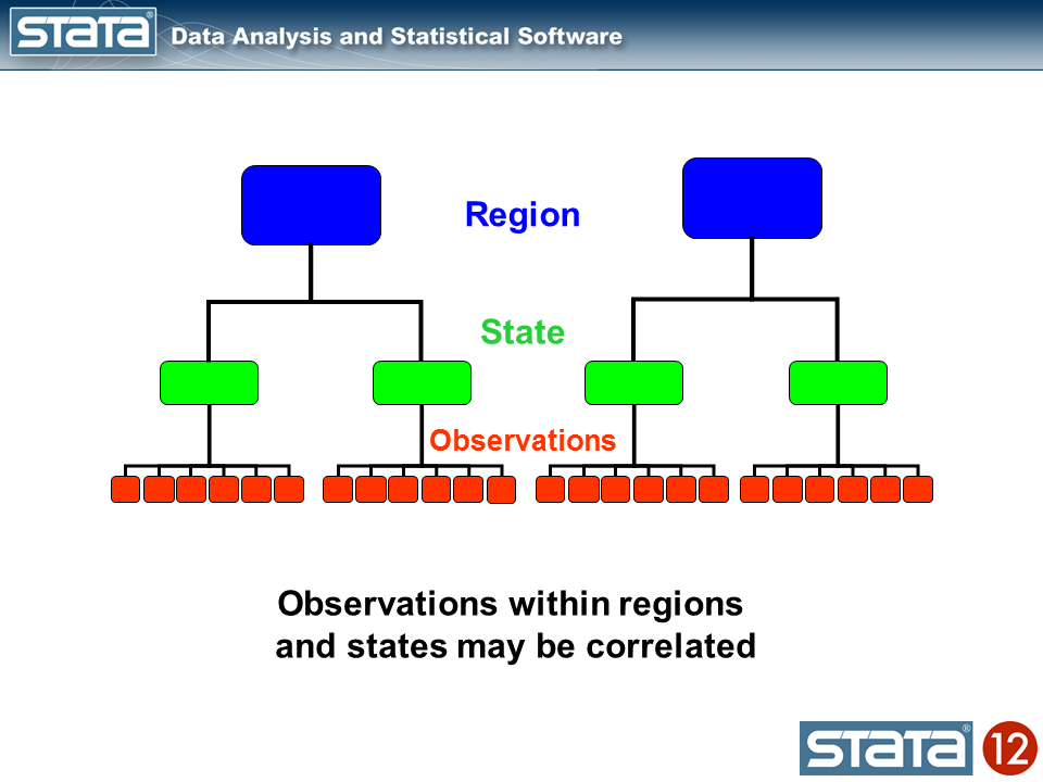
Multilevel knowledge are characterised by a hierarchical construction. A basic instance is youngsters nested inside lecture rooms and lecture rooms nested inside colleges. The take a look at scores of scholars inside the similar classroom could also be correlated because of publicity to the identical instructor or textbook. Likewise, the common take a look at scores of courses could be correlated inside a faculty because of the related socioeconomic degree of the scholars.
You could have run throughout datasets with these sorts of buildings in your individual work. For our instance, I want to use a dataset that has each longitudinal and classical hierarchical options. You possibly can entry this dataset from inside Stata by typing the next command:
use http://www.stata-press.com/knowledge/r12/productiveness.dta
We’re going to construct a mannequin of gross state product for 48 states within the USA measured yearly from 1970 to 1986. The states have been grouped into 9 areas based mostly on their financial similarity. For distributional causes, we can be modeling the logarithm of annual Gross State Product (GSP) however within the curiosity of readability, I’ll merely check with the dependent variable as GSP.
. describe gsp 12 months state area

              storage  show     worth
variable title   sort   format      label      variable label
-----------------------------------------------------------------------------
gsp             float  %9.0g                  log(gross state product)
12 months            int    %9.0g                  years 1970-1986
state           byte   %9.0g                  states 1-48
area          byte   %9.0g                  areas 1-9
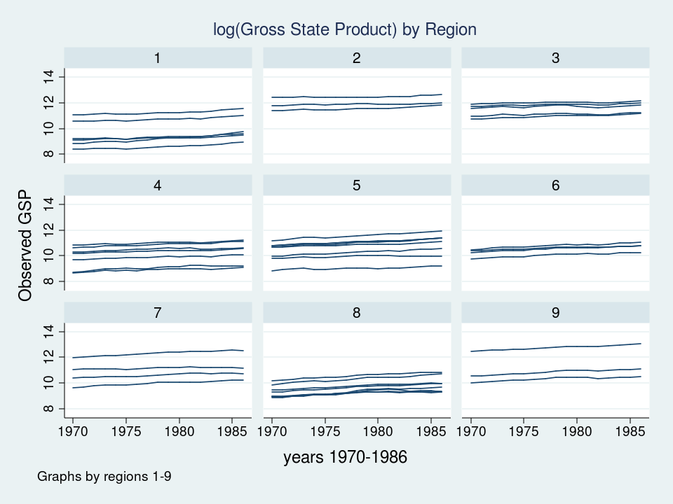
Let’s take a look at a graph of those knowledge to see what we’re working with.
twoway (line gsp 12 months, join(ascending)), ///
        by(area, title("log(Gross State Product) by Area", measurement(medsmall)))
Every line represents the trajectory of a state’s (log) GSP over time 1970 to 1986. The very first thing I discover is that the teams of strains are totally different in every of the 9 areas. Some teams of strains appear greater and a few teams appear decrease. The second factor that I discover is that the slopes of the strains will not be the identical. I’d like to include these attributes of the information into my mannequin.
Let’s sort out the vertical variations within the teams of strains first. If we take into consideration the hierarchical construction of those knowledge, I’ve repeated observations nested inside states that are in flip nested inside areas. I used shade to maintain monitor of the information hierarchy.
We may compute the imply GSP inside every state and word that the observations inside in every state range about their state imply.
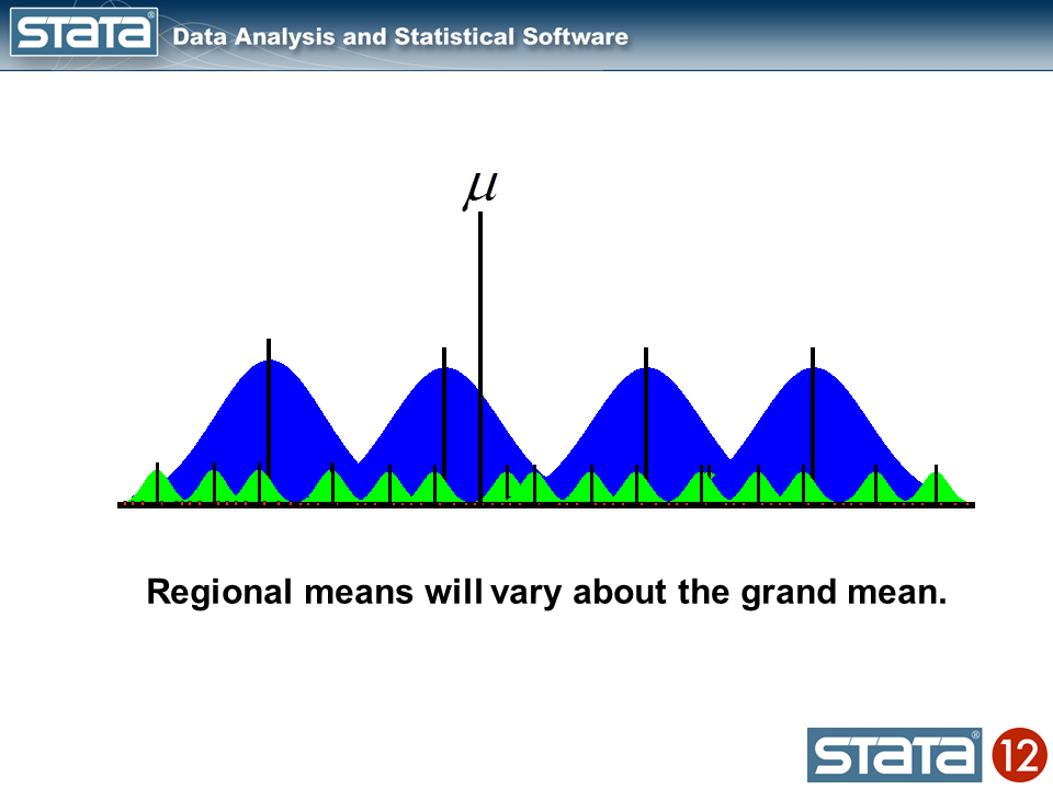
Likewise, we may compute the imply GSP inside every area and word that the state means range about their regional imply.
We may additionally compute a grand imply and word that the regional means range in regards to the grand imply.
Subsequent, let’s introduce some notation to assist us hold monitor of our mutlilevel construction. Within the jargon of multilevel modelling, the repeated measurements of GSP are described as “degree 1”, the states are known as “degree 2” and the areas are “degree 3”. I can add a three-part subscript to every statement to maintain monitor of its place within the hierarchy.
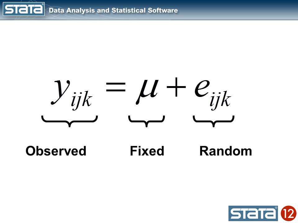
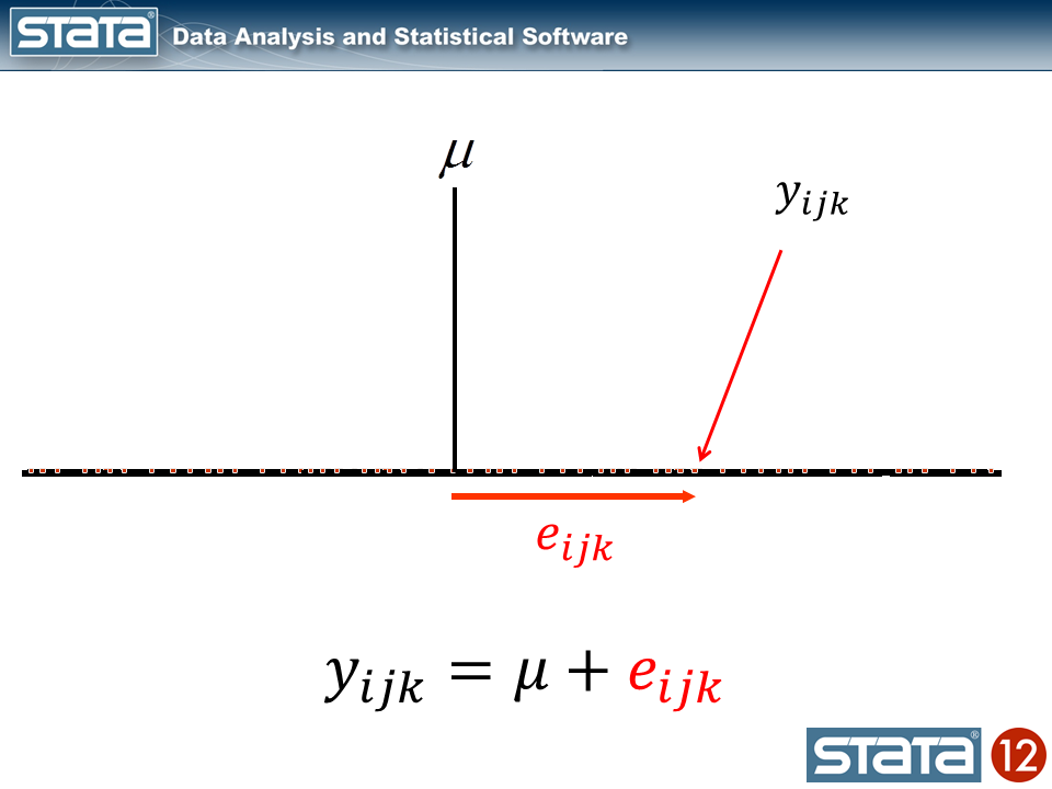
Now let’s take into consideration our mannequin. The best regression mannequin is the intercept-only mannequin which is equal to the pattern imply. The pattern imply is the “mounted” a part of the mannequin and the distinction between the statement and the imply is the residual or “random” a part of the mannequin. Econometricians typically desire the time period “disturbance”. I’m going to make use of the image μ to indicate the mounted a part of the mannequin. μ may characterize one thing so simple as the pattern imply or it may characterize a group of unbiased variables and their parameters.
Every statement can then be described when it comes to its deviation from the mounted a part of the mannequin.
If we computed this deviation of every statement, we may estimate the variability of these deviations. Let’s strive that for our knowledge utilizing Stata’s xtmixed command to suit the mannequin:
The highest desk within the output reveals the mounted a part of the mannequin which seems like another regression output from Stata, and the underside desk shows the random a part of the mannequin. Let’s take a look at a graph of our mannequin together with the uncooked knowledge and interpret our outcomes.
predict GrandMean, xb
label var GrandMean "GrandMean"
twoway  (line GrandMean 12 months, lcolor(black) lwidth(thick))              ///
        (scatter gsp 12 months, mcolor(purple) msize(tiny)),                    ///
        ytitle(log(Gross State Product), margin(medsmall))              ///
        legend(cols(4) measurement(small))                                     ///
        title("GSP for 1970-1986 by Area", measurement(medsmall))
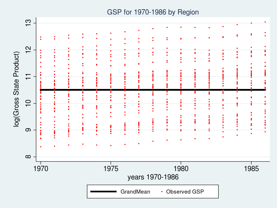
The thick black line within the middle of the graph is the estimate of _cons, which is an estimate of the mounted a part of mannequin for GSP. On this easy mannequin, _cons is the pattern imply which is the same as 10.51. In “Random-effects Parameters” part of the output, sd(Residual) is the common vertical distance between every statement (the purple dots) and glued a part of the mannequin (the black line). On this mannequin, sd(Residual) is the estimate of the pattern commonplace deviation which equals 1.02.
At this level it’s possible you’ll be considering to your self – “That’s not very fascinating – I may have completed that with Stata’s summarize command”. And you’d be right.
. summ gsp

    Variable |       Obs        Imply    Std. Dev.       Min        Max
-------------+--------------------------------------------------------
         gsp |       816    10.50885    1.021132    8.37885   13.04882
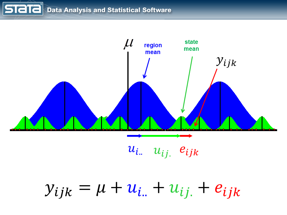
However right here’s the place it does change into fascinating. Let’s make the random a part of the mannequin extra complicated to account for the hierarchical construction of the information. Take into account a single statement, yijk and take one other take a look at its residual.
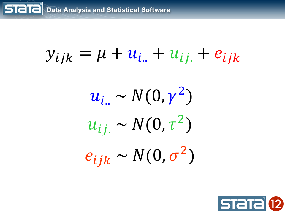
The statement deviates from its state imply by an quantity that we are going to denote eijk. The statement’s state imply deviates from the the regionals imply uij. and the statement’s regional imply deviates from the mounted a part of the mannequin, μ, by an quantity that we are going to denote ui... We have now partitioned the statement’s residual into three components, aka “elements”, that describe its magnitude relative to the state, area and grand means. If we calculated this set of residuals for every statement, wecould estimate the variability of these residuals and make distributional assumptions about them.
These sorts of fashions are sometimes referred to as “variance part” fashions as a result of they estimate the variability accounted for by every degree of the hierarchy. We will estimate a variance part mannequin for GSP utilizing Stata’s xtmixed command:
The mounted a part of the mannequin, _cons, continues to be the pattern imply. However now there are three parameters estimates within the backside desk labeled “Random-effects Parameters”. Every quantifies the common deviation at every degree of the hierarchy.
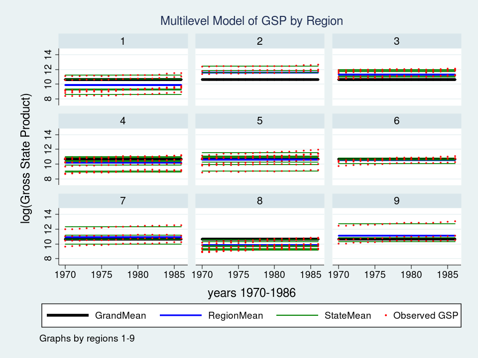
Let’s graph the predictions from our mannequin and see how effectively they match the information.
Wow – that’s a pleasant graph if I do say so myself. It could be spectacular for a report or publication, nevertheless it’s slightly powerful to learn with all 9 areas displayed directly. Let’s take a better take a look at Area 7 as a substitute.
twoway  (line GrandMean 12 months, lcolor(black) lwidth(thick))      ///
        (line RegionMean 12 months, lcolor(blue) lwidth(medthick))   ///
        (line StateMean 12 months, lcolor(inexperienced) join(ascending)) ///
        (scatter gsp 12 months, mcolor(purple) msize(medsmall))         ///
        if area ==7,                                          ///
        ytitle(log(Gross State Product), margin(medsmall))      ///
        legend(cols(4) measurement(small))                             ///
        title("Multilevel Mannequin of GSP for Area 7", measurement(medsmall))
The purple dots are the observations of GSP for every state inside Area 7. The inexperienced strains are the estimated imply GSP inside every State and the blue line is the estimated imply GSP inside Area 7. The thick black line within the middle is the general grand imply for all 9 areas. The mannequin seems to suit the information pretty effectively however I can’t assist noticing that the purple dots appear to have an upward slant to them. Our mannequin predicts that GSP is fixed inside every state and area from 1970 to 1986 when clearly the information present an upward pattern.
So we’ve tackled the primary characteristic of our knowledge. We’ve succesfully integrated the essential hierarchical construction into our mannequin by becoming a variance componentis utilizing Stata’s xtmixed command. However our graph tells us that we aren’t completed but.
Subsequent time we’ll sort out the second characteristic of our knowledge — the longitudinal nature of the observations.
If you happen to’d prefer to study extra about modelling multilevel and longitudinal knowledge, try
The following time you’re scrolling your telephone, take a second to understand the feat: The seemingly mundane act is feasible because of the coordination of 34 muscle groups, 27 joints, and over 100 tendons and ligaments in your hand. Certainly, our arms are probably the most nimble components of our our bodies. Mimicking their many nuanced gestures has been a longstanding problem in robotics and digital actuality.
Now, MIT engineers have designed an ultrasound wristband that exactly tracks a wearer’s hand actions in real-time. The wristband produces ultrasound photographs of the wrist’s muscle groups, tendons, and ligaments because the hand strikes, and is paired with a synthetic intelligence algorithm that repeatedly interprets the photographs into the corresponding positions of the 5 fingers and palm.
The researchers can prepare the wristband to study a wearer’s hand motions, which the gadget can talk in real-time to a robotic or a digital setting.
In demonstrations, the staff has proven that an individual carrying the wristband can wirelessly management a robotic hand. Because the individual gestures or factors, the robotic does the identical. In a form of wi-fi marionette interplay, the wearer can manipulate the robotic to play a easy tune on the piano and shoot a small basketball right into a desktop hoop. With the identical wristband, a wearer also can manipulate objects on a pc display screen, for example pinching their fingers collectively to enlarge and decrease a digital object.
The staff is utilizing the wristband to assemble hand movement knowledge from many extra customers with totally different hand sizes, finger shapes, and gestures. They envision constructing a big dataset of hand motions that may be plumbed, for example, to coach humanoid robots in dexterity duties, akin to performing sure surgical procedures. The ultrasound band is also used to know, manipulate, and work together with objects in video video games, design purposes, or different digital settings.
“We predict this work has quick impression in doubtlessly changing hand monitoring strategies with wearable ultrasound bands in digital and augmented actuality,” says Xuanhe Zhao, the Uncas and Helen Whitaker Professor of Mechanical Engineering at MIT. “It might additionally present big quantities of coaching knowledge for dexterous humanoid robots.”
Zhao, Gengxi Lu, and their colleagues current the wristband’s new design in a paper showing at present in Nature Electronics. Their MIT co-authors are former postdocs Xiaoyu Chen, Shucong Li, and Bolei Deng; graduate college students SeongHyeon Kim and Dian Li; postdocs Shu Wang and Runze Li; and Anantha Chandrakasan, MIT provost and the Vannevar Bush Professor of Electrical Engineering and Laptop Science. Different co-authors are graduate college students Yushun Zheng and Junhang Zhang, Baoqiang Liu, Chen Gong, and Professor Qifa Zhou from the College of Southern California.
Seeing strings
There are at present quite a lot of approaches to capturing and mimicking human hand dexterity in robots. Some approaches use cameras to document an individual’s hand actions as they manipulate objects or carry out duties. Others contain having an individual put on a glove with sensors, which information the individual’s hand actions and transmits the info to a receiving robotic. However erecting a fancy digicam system for various purposes is impractical and susceptible to visible obstacles. And sensor-laden gloves might restrict an individual’s pure hand motions and sensations.
A 3rd method makes use of {the electrical} indicators from muscle groups within the wrist or forearm that scientists then correlate with particular hand actions. Researchers have made important advances on this method, nevertheless these indicators are simply affected by noise within the setting. They’re additionally not delicate sufficient to differentiate refined modifications in actions. For example, they could discern whether or not a thumb and index finger are pinched collectively or pulled aside, however not a lot of the in-between path.
Zhao’s staff puzzled whether or not ultrasound imaging would possibly seize extra dexterous and steady hand actions. His group has been growing numerous types of ultrasound stickers — miniaturized variations of the transducers utilized in physician’s places of work which might be paired with hydrogel materials that may safely follow pores and skin.
Of their new examine, the staff included the ultrasound sticker design right into a wearable wristband to repeatedly picture the muscle groups and tendons within the wrist.
“The tendons and muscle groups in your wrist are like strings pulling on puppets, that are your fingers,” Lu says. “So the concept is: Every time you’re taking an image of the state of the strings, you’ll know the state of the hand.”
Mapping manipulation
The staff designed a wristband with an ultrasound sticker that’s the dimension of a smartwatch, and added onboard electronics which might be about as small as a cellphone. They hooked up the wristband to a volunteer’s wrist and confirmed that the gadget produced clear and steady photographs of the wrist because the volunteer moved their fingers in numerous gestures.
The problem then was to narrate the black and white ultrasound photographs of the wrist to particular positions of the hand. Because it seems, the fingers and thumb are able to 22 levels of freedom, or alternative ways of extending or angling. The researchers discovered that they may determine particular areas of their ultrasound photographs of the wrist that correlate to every of those 22 levels of freedom. For example, modifications in a single area relate to thumb extension, whereas modifications in one other area correlate with actions of the index finger.
To ascertain these connections, a volunteer carrying the wristband would transfer their hand in numerous positions whereas the researchers recorded the gestures with a number of cameras surrounding the volunteer. By matching modifications in sure areas of the ultrasound photographs with hand positions recorded by the cameras, the staff might label wrist picture areas with the corresponding diploma of freedom within the hand. However to do that translation repeatedly, and in real-time, can be an not possible activity for people.
So, the staff turned to synthetic intelligence. They used an AI algorithm that may be educated to acknowledge picture patterns and correlate them with particular labels and, on this case, the hand’s numerous levels of freedom. The researchers educated the algorithm with ultrasound photographs that they meticulously labeled, annotating the picture areas related to a particular diploma of freedom. They examined the algorithm on a brand new set of ultrasound photographs and located it appropriately predicted the corresponding hand gestures.
As soon as the researchers efficiently paired the AI algorithm with the wristband, they examined the gadget on extra volunteers. For the brand new examine, eight volunteers with totally different hand and wrist sizes wore the wristband whereas they shaped numerous hand gestures and grasps, together with making the indicators for all 26 letters in American Signal Language. In addition they held objects akin to a tennis ball, a plastic bottle, a pair of scissors, and a pencil. In every case, the wristband exactly tracked and predicted the place of the hand.
To show potential purposes, the staff developed a easy pc program that they wirelessly paired with the wristband. As a wearer went by means of the motions of pinching and greedy, the gestures corresponded to zooming out and in on an object on the pc display screen, and nearly shifting and manipulating it in a easy and steady vogue.
The researchers additionally examined the wristband as a wi-fi controller of a easy business robotic hand. Whereas carrying the wristband, a volunteer went by means of the motions of enjoying a keyboard. The robotic in flip mimicked the motions in real-time to play a easy tune on a piano. The identical robotic was additionally capable of mimic an individual’s finger faucets to play a desktop basketball sport.
Zhao is planning to additional miniaturize the wristband’s {hardware}, in addition to prepare the AI software program on many extra gestures and actions from volunteers with wider ranging hand styles and sizes. In the end, the staff is constructing towards a wearable hand tracker that may be worn by anybody, to wirelessly manipulate humanoid robots or digital objects with excessive dexterity.
“We consider that is probably the most superior strategy to observe dexterous hand movement, by means of wearable imaging of the wrist,” Zhao says. “We predict these wearable ultrasound bands can present intuitive and versatile controls for digital actuality and robotic arms.”
This analysis was supported, partly, by MIT, the U.S. Nationwide Institutes of Well being, the U.S. Nationwide Science Basis, the U.S. Division of Protection, and Singapore Nationwide Analysis Basis by means of the Singapore-MIT Alliance for Analysis and Know-how.


")


