Isaac Asimov’s three legal guidelines of robotics aren’t a sensible information
Leisure Photos/Alamy
Tremendous-intelligent synthetic intelligence rising up and wiping out humanity has been a typical trope in science fiction for many years. Now, we reside in a world the place actual AI appears to be advancing sooner than ever. Does that imply you need to begin worrying about an AI apocalypse?
Not like different existential dangers equivalent to local weather change, the dangers posed by AI are arduous to quantify. We’re in speculative territory just because we’ve a lot much less understanding of the state of affairs than we do of local weather patterns.
What we do know for sure is that lots of very sensible persons are fearful. Lots of right now’s AI firm bosses have warned of the opportunity of AI resulting in human extinction, and even the pioneer of machine intelligence, Alan Turing, spoke of a future through which computer systems turn out to be sentient, earlier than outstripping our talents and at last taking up.
The state of affairs performs out one thing like this. Think about we give an AI the only activity of fixing a giant, meaty downside just like the Riemann speculation, probably the most well-known unsolved issues in arithmetic. It may determine that what it wants is a lot and plenty of computing energy and, unconstrained by widespread sense, set about turning each inanimate object on Earth into one enormous supercomputer, leaving 8 billion of us to starve to demise in an enormous, sterile knowledge centre. It’d even use us as uncooked materials, too.
Now, you might argue that on this state of affairs, we’d discover what the AI was doing and provides it a fast nudge by saying, “By the best way, it seems to be such as you’re turning the entire world into a knowledge centre and, if that’s the case, please cease, as a result of we nonetheless have to reside on Earth.” However some individuals would possibly desire to have safeguards in place to identify this sort of situation earlier than it occurs and forestall any hurt.
Sci-fi author Isaac Asimov famously had a crack at this along with his three legal guidelines of robotics, the primary of which is {that a} robotic could not injure a human being or, by inaction, permit a human being to come back to hurt.
So, in idea, we will simply inform AI to not hurt us, and it gained’t, proper? Nicely, no. Our capacity to construct safeguards and guidelines into AI is clumsy and ineffective. We will inform right now’s massive language fashions to not be racist, or swear, or expose the recipe for explosives, however within the proper circumstances, they’ll go proper forward and do it anyway. We merely don’t perceive what occurs inside an AI mannequin effectively sufficient to forestall it doing issues we don’t need it to do.
Even when we did kind all of that out, you continue to have a state of affairs the place an AI mannequin simply decides to take us out on function – the Terminator or Matrix state of affairs. This might come about after very gradual enhancements in AI over lengthy durations, or virtually instantaneously with a singularity – the hypothetical course of whereby an AI turns into sensible sufficient to enhance itself, then quickly iterates at a fantastic tempo, getting smarter and smarter, surpassing human intelligence within the blink of an eye fixed.
And AI would possibly determine to do that as a result of it fears we’d flip it off, or as a result of it doesn’t wish to be bossed round by us, or just because it thinks Earth could be higher off with out us getting in the best way and messing issues up – a sentiment that lots of animal and plant species could effectively share in the event that they have been in a position.
It may do that through the use of an automatic biology lab to create a lethal virus, by triggering the world’s stockpile of nuclear weapons or by establishing a military of killer robots – or simply hijacking those governments are already constructing. Maybe it may even do one thing so nefarious, intelligent and sneaky that we haven’t even considered it but.
In actuality, this is likely to be difficult. An AI would possibly wish to eradicate people, however it could have restricted levers to drag. Sure, it may make all visitors lights inexperienced and take out just a few of us by way of visitors accidents. It may trigger energy outages that may get just a few extra. It may crash some planes. However taking out 8 billion individuals, abruptly? Not a straightforward activity. And it’d effectively should fend off different AI fashions which might be making an attempt to cease its murderous plans from succeeding.
Proper now, corporations with huge funding, humongous sources and groups of a number of the brightest individuals on the planet are racing to construct a superintelligent AI. Whether or not you suppose that may come quickly or not, and whether or not it can have destructive outcomes or not, we will maybe agree that if some individuals do, then it is likely to be a good suggestion to decelerate and consider carefully earlier than carrying on. Sadly, capitalism isn’t a system that’s excellent at fastidiously contemplating the results earlier than innovating, and right now’s politicians appear so eager on the potential financial upsides of AI that regulation isn’t the precedence.
So, how possible is a catastrophe? A 2024 paper that surveyed virtually 3000 revealed AI researchers revealed that greater than half thought the prospect of AI inflicting human extinction or everlasting and extreme disempowerment – the so-called p(doom) or chance of doom – was at the least 10 per cent. I don’t find out about you, however I’d actually have most popular that quantity to be a lot smaller.
Some individuals engaged on AI are optimistic in regards to the future, and a few specialists suppose it is going to be the top of humanity. Worryingly, we’re doing it anyway.
Personally, I’m of the varsity of thought that there’s nothing inherently magical in regards to the human mind and our consciousness; actually, it’s nothing that may’t be replicated artificially. So, on a protracted sufficient timescale, we’ll possible create a synthetic intelligence that vastly outstrips the flexibility of people. However I additionally suppose that we’re a protracted, great distance from understanding what that will even contain, not to mention engaging in it.
I actually don’t imagine that present fashions are wherever close to the slippery slope of a singularity – they will’t even depend to 100 reliably – and I’m not shedding sleep about the entire thing.
However – and it’s a giant however – that’s to not say that AI isn’t bringing imminent issues.
Maybe the AI apocalypse we ought to be worrying about is definitely huge job losses attributable to automation, or the gradual lack of human ability as AI takes over increasingly duties, or the additional homogenisation of tradition, stemming from AI-generated artwork, music and movie.
We lately had a contest on our Fb web page. To enter, contestants posted their favourite Stata command, characteristic, or only a submit telling us why they love Stata. Contestants then requested their pals, colleagues, and fellow Stata customers to vote for his or her entry by ‘Like’-ing the submit. The prize, a replica of Stata/MP 12 (8-core).
The response was overwhelming! We loved studying all of the the reason why customers love Stata a lot, we wished to share them with you.
The competition query was:
Do you have got a favourite command or characteristic in Stata? What a couple of memorable expertise when utilizing the software program? Publish your favourite command, characteristic, or expertise within the feedback part of this submit. Then, get your pals to “like” your remark. The individual with essentially the most “likes” by March 13, 2012, wins. The winner will obtain a single-user copy of Stata/MP8 12 with PDF documentation.
We had many submissions with a number of “likes”. The profitable submissions are:
2,235 Likes, 1st place:
Rodrigo Briceno Some of the outstanding experiences with Stata was after I realized to make use of loops. Making repetitive procedures in so quick quantities of time is de facto superb! I LIKE STATA!
1,464 Likes, 2nd place:
Juan Jose Salcedo My Favourite STATA command is by far COLLAPSE! Getting descriptive statistics couldn’t be any simpler!
140 Likes, third place:
Tymon Sloczynski My favorite command is ‘oaxaca’, a user-written command (by Ben Jann from Zurich) which can be utilized to hold out the so-called Oaxaca-Blinder decomposition. I typically use it in my analysis and it saves plenty of time – which simply makes it favorite!
Full entry listing
Mburu James inlist() February 21 at 11:28am · Like · 2.
Robin Kim exit February 21 at 11:28am · Like · 5.
Maximiliano Exequiel show !! haha.. it’s neccesary once you don’t have a calculator shut otherwise you don’t wish to open the Home windows’ calculator 🙂 February 21 at 11:31am · Like · 3.
Felipe Rojas assist February 21 at 11:31am · Like · 2.
Reynaldo Rojo Mendoza usespss. So lengthy, Stat/Switch! February 21 at 11:32am · Like · 5.
Robert Birkelbach I beloved the set reminiscence command. I miss it in Stata 12. 🙁 February 21 at 11:33am · Like · 32.
Matt Incantalupo margins February 21 at 11:33am · Like · 2.
Rodrigo Aranda di in inexperienced”¡¡VIV” in white”A ST” in purple”ATA!!” February 21 at 11:35am · Like · 9.
Emily Ryder 3 phrases: SET MORE OFF. simplistic, i do know, however let’s not faux it isn’t extraordinarily helpful when operating tabulations with tons and tons of information! February 21 at 11:39am · Like · 3.
Mike Gruszczynski foreach var of varlist x y z { do one thing } February 21 at 11:39am · Like · 4.
Peter Tennant Edit > Preferences > Common preferences > Consequence colours > Colour Scheme: Basic 🙂 February 21 at 11:43am · Like · 6.
Francisco Javier Arceo First order stochastic dominance? How do you discover out!? kdensity y, addplot( kdensity x) February 21 at 11:48am · Like · 12.
Julian Sagebiel my favourite command is ” rename ” as a result of it is extremely easy, efficient, environment friendly , no ready time and you’ll instantly observe the end result of what you probably did. particularly together with protect and restore one can have plenty of enjoyable with it February 21 at 11:48am · Like · 3.
Tihana Skrinjaric my favorite command is arch, as a result of i examine and estimate arch and garch fashions! 🙂 February 21 at 11:48am · Like · 36.
Jens Rommel world February 21 at 11:52am · Like · 4.
Sarah Bana Favourite Stata Perform: save February 21 at 11:56am · Like · 2.
Sezer Alcan my favourite command is “log” as a result of it allows me to log everthing I kind in a file February 21 at 11:59am · Like · 42.
Carrie Daymont renpfix, to alter the primary elements of all variable names that begin with the identical stub. A type of stuff you wish to do however don’t suppose there might be a command for…however there’s!!! February 21 at 12:02pm · Like · 2.
Brayan Rojas My favourite command is cond()… February 21 at 12:10pm · Like · 3.
Rafael Gralla my favourite command is assist 😉 February 21 at 12:13pm · Like · 2.
Bryce Mason Whomever made the “reshape” command must be given a medal. That command has saved me and my purchasers a boatload of money and time. February 21 at 12:15pm · Like · 70.
Rodrigo Briceño Some of the outstanding experiences with Stata was after I realized to make use of loops. Making repetitive procedures in so quick quantities of time is de facto superb! I LIKE STATA! February 21 at 12:16pm · Like · 2223.
Gabi Huiber My favourite characteristic is just not a command, however an possibility: rclass. I normally outline a program, setLocals, on the prime of the grasp do-file. Right here I outline as native macros all the things that I want to make use of in a couple of place: file paths, variable lists, title lists, constants, no matter. I name this program in every single place I want any of these items. After any given name, I solely reconstitute the actual r() outcomes that I want in that place. And if I increase the performance of my do-file and I want so as to add one other factor that might be utilized in a couple of place, I do know I solely want so as to add it within the definition of setLocals as a macro to be returned later. That’s the reason rclass is my buddy. February 21 at 12:26pm · Like · 1.
Received-ho Park All of the single-stroke instructions: d(escribe), e(xit), h(elp), m(ata), n(ote), and q(uery). February 21 at 12:42pm · Like.
Francisco Javier Arceo “Xi:” can be fairly superior when you have got an unlimited set of dummies. February 21 at 12:55pm · Like · 2.
Ryan Johnson _n and _N. Earlier than Stata, I used to be misplaced, however now I’m discovered. Database-table transformation is now little one’s play the place it as soon as was seemingly unimaginable. February 21 at 12:56pm · Like · 5.
Tymon Sloczynski My favorite command is ‘oaxaca’, a user-written command (by Ben Jann from Zurich) which can be utilized to hold out the so-called Oaxaca-Blinder decomposition. I typically use it in my analysis and it saves plenty of time – which simply makes it favorite! February 21 at 12:59pm · Like · 140.
Luca Campanelli I’m a multilevel mixed-effects individual and, for exploratory goal, it’s typically necessary to inspecting the OLS regressions for every Degree 2 unit… properly, simply run dozens of regressions, copy the coefficients of every regression, paste them in an excel file and also you’re executed. Then, at some point, the sunshine, the command -statsby-. My life modified… February 21 at 2:06pm · Like · 8.
Robert Duval H Margins is by far my favourite… A real time saver! February 21 at 2:13pm · Like · 12.
Pankaj Gaur tab is my favourite command February 21 at 2:21pm · Like.
Cristian Gil-Sánchez the most effective command ever to be taught stata is: db February 21 at 2:31pm · Like · 6.
Dmitriy Poznyak Esttab and estout save ridiculous quantity of my analysis time February 21 at 2:31pm · Like.
Sang-Min Park my funniest expertise was how the assistance file for issue variables defined interactions: “group#intercourse … identical i.group#i.intercourse”! February 21 at 2:35pm · Like · 4.
Frank MacCrory My favourite command in Stat is ‘program’, in truth Stata’s programming functionality is why I choose it over different statistics packages. Want to increase what a Stata command does? The supply code for many of them is true there so that you can use as a place to begin. February 21 at 2:55pm · Like · 3.
Juan Jose Salcedo ?….. ….. My Favourite STATA command is by far COLLAPSE! Getting descriptive statistics couldn’t be any simpler! ….. ….. February 21 at 3:06pm · Like · 1462.
Dimitriy V. Masterov Wondeing when Stata will lastly add the “gen dissertation, strong” command. February 21 at 3:25pm · Like · 21.
Norbert Schulz constraint February 21 at 4:38pm · Like · 1.
Luca Bossi My favourite command is “exit”.February 21 at 6:10pm · Like.
Stephen Merino Stata’s “reshape” command turned my selfish community information into candy, chic, dyadic information that allowed me to investigate relationship traits related to social help provision. And a shout-out to Rebekah Younger for all of her assist!! I like you, Stata. February 21 at 7:43pm · Like · 1.
Trey Marchbanks love forval x = 1/99 February 21 at 8:55pm · Like.
Jose Martinez Outreg2. Having tables and tables to format, doesn’t get higher than this. February 22 at 9:43am · Like · 1.
Habtamu Tilahun Kassahun I like the Change listing (CD) command!!! February 22 at 12:12pm · Like · 1.
Austin Nichols Favourite command? mata February 22 at 3:31pm · Like · 2.
Daniel Marcelino My favourite command is ‘egen’, its is without doubt one of the strongest although merely command of Stata. February 22 at 5:05pm · Like · 3.
Stas Kolenikov -capture-, -assert- and -confirm-, in numerous combos. You by no means know what sort of crappy information your pals, colleagues and unbiased finish customers of your packages will provide. February 22 at 6:20pm · Like · 3.
Billy Bass Apart from seconding what Stas already mentioned, I’m a giant fan of the brand new SEM capabilities and the Stata Consumer-Group as an entire. Not like another software program platforms, StataCorp and the user-community are in all probability the best asset to this system. February 22 at 6:30pm · Like · 6.
Billy Schwartz foreach var of varlist * {} rhymes properly. February 22 at 7:57pm · Like.
Chamara Anuranga My favorite command is levelsof. It’s going to retailer content material of the variable in r(varlist). It make life simpler for loop command. instance: sysuse auto.dta,clear levelsof rep78,native(listing) foreach merchandise in `listing’ { dis “`merchandise’” sum worth if rep78==`merchandise’ } I’ve used this command to attract graphs for WDI information for every nation. February 23 at 12:16am · Like · 27.
Until Da Tilt Ittermann fracpoly February 23 at 7:33am · Like · 1.
Adrian Alejandro Perez Grandes mi comando favorito es el arco, porque yo estudio y el arco y la estimación de modelos GARCH February 23 at 1:56pm · Like · 1.
Oliver Jones Have you ever ever acquired a brand new information set with no documentation and even worse BAD documentation? Simply use codebook and the solar is shining once more! 🙂 February 24 at 4:40am · Like · 14.
Marilyn Santana Reyes my favourite command is assist 😉 February 24 at 8:14am · Like · 3.
Leonardo Sanchez My favourite command is Exit. It means I’m able to go house February 24 at 9:34am · Like · 2.
Maria Gabriela Garcia Andrade ….. My Favourite STATA command is by far COLLAPSE! Getting descriptive statistics couldn’t be any simpler! ….. February 24 at 10:07pm · Like · 2.
Anayatullah Niyazi my favarate command in stata package deal is for producing new variable “gen new variable title complete(previous variable) by time” and for panel information regression “xtreg dependent variable unbiased variable , fe or re”. February 25 at 11:39am · Like.
Victor Fernandez my favorites instructions in stata are var and predict. I like attending to know the relationships between the variables after which predict how they gonna behave sooner or later. Thanks for letting me win the copy of stata! February 25 at 8:38pm · Like · 4.
Vane Ramirez Lopez Exc February 26 at 1:12am · Like · 1.
Zaira Araujo Jones exce =) February 26 at 5:47am · Like · 2.
Cecil Moitland Rodriguez the merge command is improbable! February 26 at 7:22pm · Like · 4.
Jose Francisco Pacheco-Jimenez You simply want one command: HELP! And that makes STATA the most effective of all. February 26 at 7:23pm · Like · 4.
Reymond Ssr regress rocks February 26 at 7:25pm · Like · 1.
David Mora G is without doubt one of the greatest instructions please vote for me.. February 26 at 7:26pm · Like · 1.
Alejandra Hernández tab is the most effective command of Stata… February 26 at 7:30pm · Like · 1.
David Lang my favourite command is internet search, because it permits me entry to all the brand new procedures. February 27 at 1:26pm · Like · 4.
Jason Gainous My favourite command is whichever one I’ve to lookup subsequent on the Google. February 27 at 11:10pm · Like · 44.
Víctor Hugo Pérez My favourite command? Uhhh, that’s a tough one… I’ll guess it’s foreach… It’s the extra versatile and time-saving command I’ve ever used. It’s straightforward to make use of and allows you to keep away from numerous boring programming. February 28 at 2:38pm · Like · 27.
David Elliott When it’s a must to do some repetitive heavy lifting there’s nothing higher than: levelsof x, native(xlevels) foreach degree of native xlevels { …`degree’… } February 28 at 2:42pm · Like · 3.
Niki Yang My favourite command is “DIsplay 1+1” which is a good substitute for a pocket calculator! For all the things else, I take advantage of Mata! February 28 at 2:53pm · Like · 4.
Tobin Hanspal estout! February 28 at 2:55pm · Like · 1.
Adrian Mander Exit,clear. It means it’s house time February 28 at 4:34pm · Like · 3.
Tomek Godlewski Management alt delete. February 28 at 6:40pm · Like · 2.
Alberto Dorantes My favourite command: for information administration: collapse (way more environment friendly than PivotTables of Excel), and for information evaluation the pre-command: rolling, which saves tons of programming strains February 28 at 6:48pm · Like · 3.
Denier Duarte Alvarado Exit clear.. February 28 at 9:51pm · Like · 1.
Hiroshi Kameyama now utilizing many instances, “arfima”, what occur subsequent? February 29 at 1:48am · Like.
Antoinette Post-mortem My Favourite STATA command is collapse. February 29 at 10:47am · Like · 91.
Korin Esquivel listo ! February 29 at 2:34pm · Like · 2.
Cirito Moran Contreras dame tu pin x interno February 29 at 3:25pm · Like · 1.
Stata person foreach and forvalus are each nice conmands,i really like them February 29 at 4:59pm · Like · 1.
Marcelo Lopez Leon DEMACIADAS XUERTE March 1 at 4:04pm · Like · 1.
Aguirrense Rafiko De Corazon Zambrano ps xq tanto ingles March 1 at 7:07pm · Like · 2.
Ines Bouassida My favourite command is “merge” March 5 at 12:43pm · Like · 38.
Chase Coleman I feel my favo makes creating binary variables fast and easy March 5 at 11:37pm · Like · 18.
Juliana Camacho Sánchez my favourite command is assist March 6 at 12:38pm · Like · 5.
Vicki Stagg My favourite Stata information manipulation software combines using _n and subscripting.The next do-file might be utilized to affected person information over numerous numbers of visits. Enter information would come with affected person ids, go to dates and systolic BP measurements, for instance. A affected person sequence quantity and baseline (from the primary go to) systolic BP worth are generated and utilized to every report. type patientid visitdt bysort patientid: gen seq_visit=_n bysort patientid: gen tot_visit=_N *tabulate the variety of visits tab tot_visit if seq_visit==tot_visit *put together to generate affected person sequence quantity and baseline sys bp type seq_visit patientid gen patientn=_n if seq_visit==1 gen base_bpsys = bp_sys if seq_visit==1 type patientid seq_visit bysort patientid: change patientn=patientn[1] bysort patientid: change base_bpsys= base_bpsys[1] March 9 at 4:29am · Like · 7.
Christopher Salazar me gusta propio viejo Saturday at 2:16pm · Like.
Liu Pluas Diaz propio pepa Saturday at 3:50pm · Like.
Mariel García M I see two individuals who introduced over a thousand likes every to this standing replace. I hope the corporate will admire that and provides them each a free copy. Statisticians don’t get that a lot help on a regular basis! Sunday at 11:45pm · Like · 1.
Alexander A. Stäubert I bought this reply after operating the GLLAMM command: “can’t get appropriate log-likelihood: -39386.119 must be -39386.664. one thing went unsuitable in comprob3”. Normally Stata may be very exact when stating an error… normally. Yesterday at 11:59am · Like.
Rajesh Tharyan my favorite command is ! which lets you ship instructions to your working system or to enter your working system for interactive use, !!..:) Yesterday at 12:01pm · Like · 1.
Nguyen Ngoc Quang My favourite command is subinstr to transform the unicode font Yesterday at 12:04pm · Like · 1.
Juan Pablo Ocampo Years in the past whereas doing an econometrics homework I had plenty of hassle with a dummy entice. Immediately a buddy prompt to make use of “tetrachoric” to verify correlation between dummies. I’m in love with that command since, additionally it’s enjoyable to say it…tetrachoric 23 hours in the past · Like · 1.
Gülsün Akin It will be nice if these feedback might be saved someplace.. I’ve realized a number of issues to make life simpler by searching some, and wish to learn all sooner or later. 23 hours in the past · Not like · 1.
Andrew Dyck My favorite command is -reshape-. This is a gigantic ache in most statistical frameworks, however sooo straightforward with STATA. Sustain the good work! 20 hours in the past · Like · 3.
Ronald Moreano Que El Señor Dios Jehova te bendiga, guie tu camino e ilumine tu vida por siempre. 14 hours in the past · Like · 1.
Minh Nguyen My favorite command is egen with bysort. 12 hours in the past · Like.
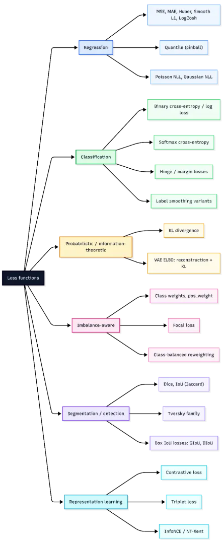
A loss operate is what guides a mannequin throughout coaching, translating predictions right into a sign it could actually enhance on. However not all losses behave the identical—some amplify giant errors, others keep secure in noisy settings, and every selection subtly shapes how studying unfolds.
Trendy libraries add one other layer with discount modes and scaling results that affect optimization. On this article, we break down the foremost loss households and the way to decide on the suitable one on your job.
Mathematical Foundations of Loss Features
In supervised studying, the target is often to attenuate the empirical threat,
(typically with elective pattern weights and regularization).
the place ℓ is the loss operate, fθ(xi) is the mannequin prediction, and yi is the true goal. In apply, this goal can also embody pattern weights and regularization phrases. Most machine studying frameworks comply with this formulation by computing per-example losses after which making use of a discount corresponding to imply, sum, or none.
When discussing mathematical properties, it is very important state the variable with respect to which the loss is analyzed. Many loss features are convex within the prediction or logit for a set label, though the general coaching goal is normally non-convex in neural community parameters. Necessary properties embody convexity, differentiability, robustness to outliers, and scale sensitivity. Frequent implementation of pitfalls contains complicated logits with chances and utilizing a discount that doesn’t match the meant mathematical definition.
Regression Losses
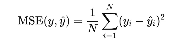
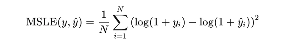
Imply Squared Error
Imply Squared Error, or MSE, is without doubt one of the most generally used loss features for regression. It’s outlined as the typical of the squared variations between predicted values and true targets:
As a result of the error time period is squared, giant residuals are penalized extra closely than small ones. This makes MSE helpful when giant prediction errors needs to be strongly discouraged. It’s convex within the prediction and differentiable all over the place, which makes optimization easy. Nonetheless, it’s delicate to outliers, since a single excessive residual can strongly have an effect on the loss.
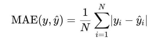
Imply Absolute Error, or MAE, measures the typical absolute distinction between predictions and targets:
Not like MSE, MAE penalizes errors linearly fairly than quadratically. In consequence, it’s extra sturdy to outliers. MAE is convex within the prediction, however it isn’t differentiable at zero residual, so optimization usually makes use of subgradients at that time.
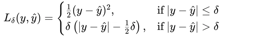
Huber loss combines the strengths of MSE and MAE by behaving quadratically for small errors and linearly for big ones. For a threshold δ>0, it’s outlined as:
This makes Huber loss a sensible choice when the information are largely effectively behaved however might include occasional outliers.
Easy L1 loss is carefully associated to Huber loss and is often utilized in deep studying, particularly in object detection and regression heads. It transitions from a squared penalty close to zero to an absolute penalty past a threshold. It’s differentiable all over the place and fewer delicate to outliers than MSE.
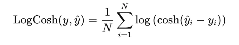
Log-cosh loss is a clean different to MAE and is outlined as
Close to zero residuals, it behaves like squared loss, whereas for big residuals it grows nearly linearly. This provides it an excellent stability between clean optimization and robustness to outliers.
Quantile loss, additionally referred to as pinball loss, is used when the aim is to estimate a conditional quantile fairly than a conditional imply. For a quantile stage τ∈(0,1) and residual u=y−y^ it’s outlined as
It penalizes overestimation and underestimation asymmetrically, making it helpful in forecasting and uncertainty estimation.
import numpy as np

y_true = np.array([3.0, -0.5, 2.0, 7.0])
y_pred = np.array([2.5, 0.0, 2.0, 8.0])

tau = 0.8

u = y_true - y_pred

quantile_loss = np.imply(np.the place(u >= 0, tau * u, (tau - 1) * u))

print("Quantile Loss:", quantile_loss)
import numpy as np

y_true = np.array([3.0, -0.5, 2.0, 7.0])
y_pred = np.array([2.5, 0.0, 2.0, 8.0])

tau = 0.8

u = y_true - y_pred

quantile_loss = np.imply(np.the place(u >= 0, tau * u, (tau - 1) * u))

print("Quantile Loss:", quantile_loss)
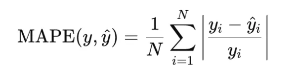
MAPE
Imply Absolute Proportion Error, or MAPE, measures relative error and is outlined as
It’s helpful when relative error issues greater than absolute error, but it surely turns into unstable when goal values are zero or very near zero.
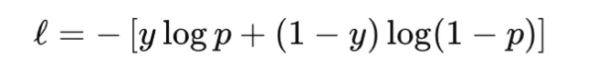
Binary cross-entropy, or BCE, is used for binary classification. It compares a Bernoulli label y∈{0,1} with a predicted chance p∈(0,1):
In apply, many libraries want logits fairly than chances and compute the loss in a numerically secure approach. This avoids instability brought on by making use of sigmoid individually earlier than the logarithm. BCE is convex within the logit for a set label and differentiable, however it isn’t sturdy to label noise as a result of confidently improper predictions can produce very giant loss values. It’s broadly used for binary classification, and in multi-label classification it’s utilized independently to every label. A typical pitfall is complicated chances with logits, which might silently degrade coaching.
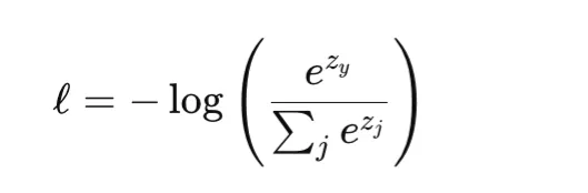
Softmax Cross-Entropy for Multiclass Classification
Softmax cross-entropy is the usual loss for multiclass classification. For a category index y and logits vector z, it combines the softmax transformation with cross-entropy loss:
This loss is convex within the logits and differentiable. Like BCE, it could actually closely penalize assured improper predictions and isn’t inherently sturdy to label noise. It’s generally utilized in commonplace multiclass classification and likewise in pixelwise classification duties corresponding to semantic segmentation. One necessary implementation element is that many libraries, together with PyTorch, anticipate integer class indices fairly than one-hot targets until soft-label variants are explicitly used.
import torch
import torch.nn.purposeful as F

logits = torch.tensor([
    [2.0, 0.5, -1.0],
    [0.0, 1.0, 0.0]
], dtype=torch.float32)

y_true = torch.tensor([0, 2], dtype=torch.lengthy)

loss = F.cross_entropy(logits, y_true)

print("CrossEntropyLoss:", loss.merchandise())
Label Smoothing Variant
Label smoothing is a regularized type of cross-entropy during which a one-hot goal is changed by a softened goal distribution. As a substitute of assigning full chance mass to the proper class, a small portion is distributed throughout the remaining courses. This discourages overconfident predictions and might enhance calibration.
The tactic stays differentiable and infrequently improves generalization, particularly in large-scale classification. Nonetheless, an excessive amount of smoothing could make the targets overly ambiguous and result in underfitting.
import torch
import torch.nn.purposeful as F

logits = torch.tensor([
    [2.0, 0.5, -1.0],
    [0.0, 1.0, 0.0]
], dtype=torch.float32)

y_true = torch.tensor([0, 2], dtype=torch.lengthy)

loss = F.cross_entropy(logits, y_true, label_smoothing=0.1)

print("CrossEntropyLoss with label smoothing:", loss.merchandise())
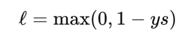
Margin Losses: Hinge Loss
Hinge loss is a basic margin-based loss utilized in help vector machines. For binary classification with label y∈{−1,+1} and rating s, it’s outlined as
Hinge loss is convex within the rating however not differentiable on the margin boundary. It produces zero loss for examples which might be appropriately categorised with adequate margin, which results in sparse gradients. Not like cross-entropy, hinge loss shouldn’t be probabilistic and doesn’t straight present calibrated chances. It’s helpful when a max-margin property is desired.
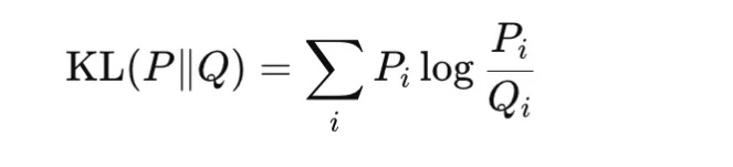
Kullback-Leibler divergence compares two chance distributions P and Q:
It’s nonnegative and turns into zero solely when the 2 distributions are similar. KL divergence shouldn’t be symmetric, so it isn’t a real metric. It’s broadly utilized in information distillation, variational inference, and regularization of realized distributions towards a previous. In apply, PyTorch expects the enter distribution in log-probability type, and utilizing the improper discount can change the reported worth. Specifically, batchmean matches the mathematical KL definition extra carefully than imply.
import torch
import torch.nn.purposeful as F

P = torch.tensor([[0.7, 0.2, 0.1]], dtype=torch.float32)
Q = torch.tensor([[0.6, 0.3, 0.1]], dtype=torch.float32)

kl_batchmean = F.kl_div(Q.log(), P, discount="batchmean")

print("KL Divergence (batchmean):", kl_batchmean.merchandise())
KL Divergence Discount Pitfall
A typical implementation problem with KL divergence is the selection of discount. In PyTorch, discount=”imply” scales the consequence otherwise from the true KL expression, whereas discount=”batchmean” higher matches the usual definition.
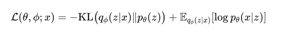
The variational autoencoder, or VAE, is skilled by maximizing the proof decrease certain, generally referred to as the ELBO:
This goal has two components. The reconstruction time period encourages the mannequin to elucidate the information effectively, whereas the KL time period regularizes the approximate posterior towards the prior. The ELBO shouldn’t be convex in neural community parameters, however it’s differentiable underneath the reparameterization trick. It’s broadly utilized in generative modeling and probabilistic illustration studying. In apply, many variants introduce a weight on the KL time period, corresponding to in beta-VAE.
Class weighting is a typical technique for dealing with imbalanced datasets. As a substitute of treating all courses equally, increased loss weight is assigned to minority courses in order that their errors contribute extra strongly throughout coaching. In multiclass classification, weighted cross-entropy is usually used:
the place wy is the load for the true class. This method is easy and efficient when class frequencies differ considerably. Nonetheless, excessively giant weights could make optimization unstable.
For binary or multi-label classification, many libraries present a pos_weight parameter that will increase the contribution of optimistic examples in binary cross-entropy. That is particularly helpful when optimistic labels are uncommon. In PyTorch, BCEWithLogitsLoss helps this straight.
This methodology is usually most well-liked over naive resampling as a result of it preserves all examples whereas adjusting the optimization sign. A typical mistake is to confuse weight and pos_weight, since they have an effect on the loss otherwise.
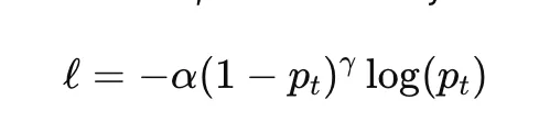
Focal loss is designed to handle class imbalance by down-weighting straightforward examples and focusing coaching on tougher ones. For binary classification, it’s generally written as
the place pt is the mannequin chance assigned to the true class, α is a class-balancing issue, and γ controls how strongly straightforward examples are down-weighted. When γ=0, focal loss reduces to unusual cross-entropy.
Focal loss is broadly utilized in dense object detection and extremely imbalanced classification issues. Its predominant hyperparameters are α and γ, each of which might considerably have an effect on coaching habits.
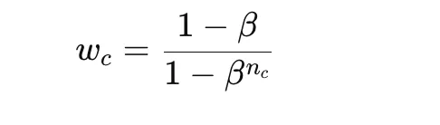
Class-balanced reweighting improves on easy inverse-frequency weighting through the use of the efficient variety of samples fairly than uncooked counts. A typical system for the category weight is
the place nc is the variety of samples in school c and β is a parameter near 1. This provides smoother and infrequently extra secure reweighting than direct inverse counts.
This methodology is helpful when class imbalance is extreme however naive class weights could be too excessive. The primary hyperparameter is β, which determines how strongly uncommon courses are emphasised.
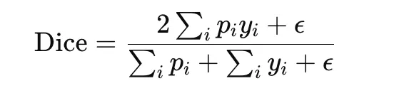
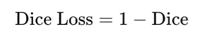
Cube loss is broadly utilized in picture segmentation, particularly when the goal area is small relative to the background. It’s primarily based on the Cube coefficient, which measures overlap between the expected masks and the ground-truth masks:
The corresponding loss is
Cube loss straight optimizes overlap and is subsequently effectively suited to imbalanced segmentation duties. It’s differentiable when smooth predictions are used, however it may be delicate to small denominators, so a smoothing fixed ϵ is normally added.
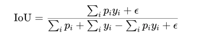
Intersection over Union, or IoU, additionally referred to as Jaccard index, is one other overlap-based measure generally utilized in segmentation and detection. It’s outlined as
The loss type is
IoU loss is stricter than Cube loss as a result of it penalizes disagreement extra strongly. It’s helpful when correct area overlap is the primary goal. As with Cube loss, a small fixed is added for stability.
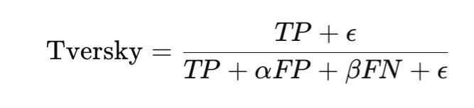
Tversky loss generalizes Cube and IoU type overlap losses by weighting false positives and false negatives otherwise. The Tversky index is
and the loss is
This makes it particularly helpful in extremely imbalanced segmentation issues, corresponding to medical imaging, the place lacking a optimistic area could also be a lot worse than together with further background. The selection of α and β controls this tradeoff.
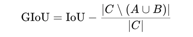
Generalized IoU, or GIoU, is an extension of IoU designed for bounding-box regression in object detection. Customary IoU turns into zero when two bins don’t overlap, which provides no helpful gradient. GIoU addresses this by incorporating the smallest enclosing field CCC:
The loss is
GIoU is helpful as a result of it nonetheless gives a coaching sign even when predicted and true bins don’t overlap.
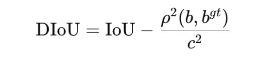
Distance IoU, or DIoU, extends IoU by including a penalty primarily based on the gap between field facilities. It’s outlined as
the place ρ2(b,bgt) is the squared distance between the facilities of the expected and ground-truth bins, and c2 is the squared diagonal size of the smallest enclosing field. The loss is
DIoU improves optimization by encouraging each overlap and spatial alignment. It’s generally utilized in bounding-box regression for object detection.
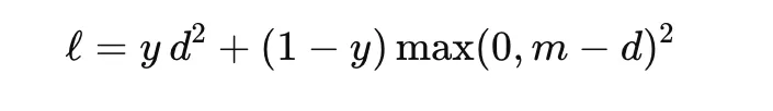
Contrastive loss is used to be taught embeddings by bringing comparable samples nearer collectively and pushing dissimilar samples farther aside. It’s generally utilized in Siamese networks. For a pair of embeddings with distance d and label y∈{0,1}, the place y=1 signifies an identical pair, a typical type is
the place m is the margin. This loss encourages comparable pairs to have small distance and dissimilar pairs to be separated by no less than the margin. It’s helpful in face verification, signature matching, and metric studying.
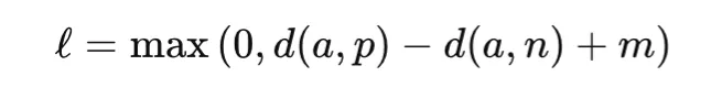
Triplet loss extends pairwise studying through the use of three examples: an anchor, a optimistic pattern from the identical class, and a detrimental pattern from a distinct class. The target is to make the anchor nearer to the optimistic than to the detrimental by no less than a margin:
the place d(⋅, ⋅) is a distance operate and m is the margin. Triplet loss is broadly utilized in face recognition, individual re-identification, and retrieval of duties. Its success relies upon strongly on how informative triplets are chosen throughout coaching.
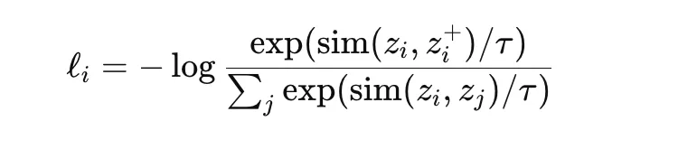
InfoNCE is a contrastive goal broadly utilized in self-supervised illustration studying. It encourages an anchor embedding to be near its optimistic pair whereas being removed from different samples within the batch, which act as negatives. A normal type is
the place sim is a similarity measure corresponding to cosine similarity and τ is a temperature parameter. NT-Xent is a normalized temperature-scaled variant generally utilized in strategies corresponding to SimCLR. These losses are highly effective as a result of they be taught wealthy representations with out guide labels, however they rely strongly on batch composition, augmentation technique, and temperature selection.
import torch
import torch.nn.purposeful as F

z_anchor = torch.tensor([[1.0, 0.0]], dtype=torch.float32)
z_positive = torch.tensor([[0.9, 0.1]], dtype=torch.float32)
z_negative1 = torch.tensor([[0.0, 1.0]], dtype=torch.float32)
z_negative2 = torch.tensor([[-1.0, 0.0]], dtype=torch.float32)

embeddings = torch.cat([z_positive, z_negative1, z_negative2], dim=0)

z_anchor = F.normalize(z_anchor, dim=1)
embeddings = F.normalize(embeddings, dim=1)

similarities = torch.matmul(z_anchor, embeddings.T).squeeze(0)

temperature = 0.1
logits = similarities / temperature

labels = torch.tensor([0], dtype=torch.lengthy)  # optimistic is first

loss = F.cross_entropy(logits.unsqueeze(0), labels)

print("InfoNCE / NT-Xent Loss:", loss.merchandise())
Comparability Desk and Sensible Steerage
The desk beneath summarizes key properties of generally used loss features. Right here, convexity refers to convexity with respect to the mannequin output, corresponding to prediction or logit, for fastened targets, not convexity in neural community parameters. This distinction is necessary as a result of most deep studying targets are non-convex in parameters, even when the loss is convex within the output.
Loss
Typical Activity
Convex in Output
Differentiable
Sturdy to Outliers
Scale / Models
MSE
Regression
Sure
Sure
No
Squared goal items
MAE
Regression
Sure
No (kink)
Sure
Goal items
Huber
Regression
Sure
Sure
Sure (managed by δ)
Goal items
Easy L1
Regression / Detection
Sure
Sure
Sure
Goal items
Log-cosh
Regression
Sure
Sure
Reasonable
Goal items
Pinball (Quantile)
Regression / Forecast
Sure
No (kink)
Sure
Goal items
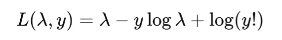
Poisson NLL
Rely Regression
Sure (λ>0)
Sure
Not major focus
Nats
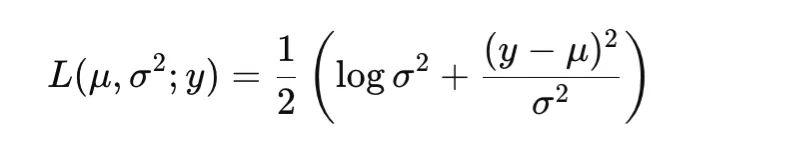
Gaussian NLL
Uncertainty Regression
Sure (imply)
Sure
Not major focus
Nats
BCE (logits)
Binary / Multilabel
Sure
Sure
Not relevant
Nats
Softmax Cross-Entropy
Multiclass
Sure
Sure
Not relevant
Nats
Hinge
Binary / SVM
Sure
No (kink)
Not relevant
Margin items
Focal Loss
Imbalanced Classification
Usually No
Sure
Not relevant
Nats
KL Divergence
Distillation / Variational
Context-dependent
Sure
Not relevant
Nats
Cube Loss
Segmentation
No
Virtually (smooth)
Not major focus
Unitless
IoU Loss
Segmentation / Detection
No
Virtually (smooth)
Not major focus
Unitless
Tversky Loss
Imbalanced Segmentation
No
Virtually (smooth)
Not major focus
Unitless
GIoU
Field Regression
No
Piecewise
Not major focus
Unitless
DIoU
Field Regression
No
Piecewise
Not major focus
Unitless
Contrastive Loss
Metric Studying
No
Piecewise
Not major focus
Distance items
Triplet Loss
Metric Studying
No
Piecewise
Not major focus
Distance items
InfoNCE / NT-Xent
Contrastive Studying
No
Sure
Not major focus
Nats
Conclusion
Loss features outline how fashions measure error and be taught throughout coaching. Totally different duties—regression, classification, segmentation, detection, and illustration studying—require totally different loss varieties. Selecting the best one relies on the issue, knowledge distribution, and error sensitivity. Sensible concerns like numerical stability, gradient scale, discount strategies, and sophistication imbalance additionally matter. Understanding loss features results in higher coaching and extra knowledgeable mannequin design selections.
Often Requested Questions
Q1. What does a loss operate do in machine studying?
A. It measures the distinction between predictions and true values, guiding the mannequin to enhance throughout coaching.
Q2. How do I select the suitable loss operate?
A. It relies on the duty, knowledge distribution, and which errors you wish to prioritize or penalize.
Q3. Why do discount strategies matter?
A. They have an effect on gradient scale, influencing studying price, stability, and total coaching habits.
Hello, I’m Janvi, a passionate knowledge science fanatic presently working at Analytics Vidhya. My journey into the world of knowledge started with a deep curiosity about how we will extract significant insights from complicated datasets.
Login to proceed studying and revel in expert-curated content material.
We’ve all turn into used to deep studying’s success in picture classification. Better Swiss Mountain canine or Bernese mountain canine? Crimson panda or big panda? No drawback.
Nonetheless, in actual life it’s not sufficient to call the one most salient object on an image. Prefer it or not, one of the vital compelling examples is autonomous driving: We don’t need the algorithm to acknowledge simply that automobile in entrance of us, but in addition the pedestrian about to cross the road. And, simply detecting the pedestrian shouldn’t be adequate. The precise location of objects issues.
The time period object detection is often used to confer with the duty of naming and localizing a number of objects in a picture body. Object detection is tough; we’ll construct as much as it in a free collection of posts, specializing in ideas as a substitute of aiming for final efficiency. At the moment, we’ll begin with just a few simple constructing blocks: Classification, each single and a number of; localization; and mixing each classification and localization of a single object.
Dataset
We’ll be utilizing photos and annotations from the Pascal VOC dataset which might be downloaded from this mirror.
Particularly, we’ll use knowledge from the 2007 problem and the identical JSON annotation file as used within the quick.ai course.
In phrases, we take the photographs and the annotation file from totally different locations:
Whether or not you’re executing the listed instructions or arranging information manually, you need to finally find yourself with directories/information analogous to those:
Checklist of 4
 $ photos     :Checklist of 2501
 $ kind       : chr "cases"
 $ annotations:Checklist of 7844
 $ classes :Checklist of 20
First, traits of the picture itself (peak and width) and the place it’s saved. Not surprisingly, right here it’s one entry per picture.
Then, object class ids and bounding field coordinates. There could also be a number of of those per picture.
In Pascal VOC, there are 20 object lessons, from ubiquitous automobiles (automobile, aeroplane) over indispensable animals (cat, sheep) to extra uncommon (in widespread datasets) varieties like potted plant or television monitor.
For the bounding bins, the annotation file offers x_left and y_top coordinates, in addition to width and peak.
We are going to largely be working with nook coordinates, so we create the lacking x_right and y_bottom.
As normal in picture processing, the y axis begins from the highest.
Lastly, we nonetheless have to match class ids to class names.
So, placing all of it collectively:
Observe that right here nonetheless, we’ve a number of entries per picture, every annotated object occupying its personal row.
There’s one step that may bitterly damage our localization efficiency if we later overlook it, so let’s do it now already: We have to scale all bounding field coordinates in line with the precise picture dimension we’ll use once we move it to our community.
Now as indicated above, on this submit we’ll largely tackle dealing with a single object in a picture. This implies we’ve to determine, per picture, which object to single out.
An inexpensive technique appears to be selecting the thing with the most important floor fact bounding field.
After this operation, we solely have 2501 photos to work with – not many in any respect! For classification, we may merely use knowledge augmentation as offered by Keras, however to work with localization we’d should spin our personal augmentation algorithm.
We’ll depart this to a later event and for now, give attention to the fundamentals.
our coaching set consists of 2000 photos with one annotation every. We’re prepared to start out coaching, and we’ll begin gently, with single-object classification.
Single-object classification
In all instances, we’ll use XCeption as a primary characteristic extractor. Having been educated on ImageNet, we don’t count on a lot wonderful tuning to be essential to adapt to Pascal VOC, so we depart XCeption’s weights untouched
How ought to we move our knowledge to Keras? We may easy use Keras’ image_data_generator, however given we’ll want customized turbines quickly, we’ll construct a easy one ourselves.
This one delivers photos in addition to the corresponding targets in a stream. Observe how the targets will not be one-hot-encoded, however integers – utilizing sparse_categorical_crossentropy as a loss perform allows this comfort.
For us, after 8 epochs, accuracies on the prepare resp. validation units had been at 0.68 and 0.74, respectively. Not too unhealthy given given we’re attempting to distinguish between 20 lessons right here.
Now let’s shortly assume what we’d change if we had been to categorise a number of objects in a single picture. Adjustments largely concern preprocessing steps.
A number of object classification
This time, we multi-hot-encode our knowledge. For each picture (as represented by its filename), right here we’ve a vector of size 20 the place 0 signifies absence, 1 means presence of the respective object class:
image_cats<-imageinfo%>%choose(category_id)%>%mutate(category_id =category_id-1)%>%pull()%>%to_categorical(num_classes =20)image_cats<-knowledge.body(image_cats)%>%add_column(file_name =imageinfo$file_name, .earlier than =TRUE)image_cats<-image_cats%>%group_by(file_name)%>%summarise_all(.funs =funs(max))n_samples<-nrow(image_cats)train_indices<-pattern(1:n_samples, 0.8*n_samples)train_data<-image_cats[train_indices,]validation_data<-image_cats[-train_indices,]
Correspondingly, we modify the generator to return a goal of dimensions batch_size * 20, as a substitute of batch_size * 1.
Now, essentially the most fascinating change is to the mannequin – although it’s a change to 2 strains solely.
Had been we to make use of categorical_crossentropy now (the non-sparse variant of the above), mixed with a softmax activation, we might successfully inform the mannequin to select only one, particularly, essentially the most possible object.
As an alternative, we wish to determine: For every object class, is it current within the picture or not? Thus, as a substitute of softmax we use sigmoid, paired with binary_crossentropy, to acquire an unbiased verdict on each class.
This time, (binary) accuracy surpasses 0.95 after one epoch already, on each the prepare and validation units. Not surprisingly, accuracy is considerably larger right here than once we needed to single out certainly one of 20 lessons (and that, with different confounding objects current generally!).
Now, likelihood is that if you happen to’ve accomplished any deep studying earlier than, you’ve accomplished picture classification in some type, maybe even within the multiple-object variant. To construct up within the path of object detection, it’s time we add a brand new ingredient: localization.
Single-object localization
From right here on, we’re again to coping with a single object per picture. So the query now could be, how can we study bounding bins?
In case you’ve by no means heard of this, the reply will sound unbelievably easy (naive even): We formulate this as a regression drawback and intention to foretell the precise coordinates. To set practical expectations – we certainly shouldn’t count on final precision right here. However in a method it’s superb it does even work in any respect.
What does this imply, formulate as a regression drawback? Concretely, it means we’ll have a dense output layer with 4 items, every comparable to a nook coordinate.
So let’s begin with the mannequin this time. Once more, we use Xception, however there’s an essential distinction right here: Whereas earlier than, we stated pooling = "avg" to acquire an output tensor of dimensions batch_size * variety of filters, right here we don’t do any averaging or flattening out of the spatial grid. It’s because it’s precisely the spatial data we’re focused on!
For Xception, the output decision might be 7×7. So a priori, we shouldn’t count on excessive precision on objects a lot smaller than about 32×32 pixels (assuming the usual enter dimension of 224×224).
We are going to prepare with one of many loss capabilities frequent in regression duties, imply absolute error. However in duties like object detection or segmentation, we’re additionally focused on a extra tangible amount: How a lot do estimate and floor fact overlap?
Overlap is normally measured as Intersection over Union, or Jaccard distance. Intersection over Union is strictly what it says, a ratio between area shared by the objects and area occupied once we take them collectively.
To evaluate the mannequin’s progress, we are able to simply code this as a customized metric:
After 8 epochs, IOU on each coaching and take a look at units is round 0.35. This quantity doesn’t look too good. To study extra about how coaching went, we have to see some predictions. Right here’s a comfort perform that shows a picture, the bottom fact field of essentially the most salient object (as outlined above), and if given, class and bounding field predictions.
Pattern bounding field predictions on the coaching set.
As you’d guess from wanting, the cyan-colored bins are the bottom fact ones. Now wanting on the predictions explains quite a bit in regards to the mediocre IOU values! Let’s take the very first pattern picture – we needed the mannequin to give attention to the couch, but it surely picked the desk, which can be a class within the dataset (though within the type of eatingdesk). Comparable with the picture on the precise of the primary row – we needed to it to select simply the canine but it surely included the particular person, too (by far essentially the most steadily seen class within the dataset).
So we truly made the duty much more tough than had we stayed with e.g., ImageNet the place usually a single object is salient.
Now verify predictions on the validation set.
Some bounding field predictions on the validation set.
Once more, we get an identical impression: The mannequin did study one thing, however the process is sick outlined. Have a look at the third picture in row 2: Isn’t it fairly consequent the mannequin picks all folks as a substitute of singling out some particular man?
If single-object localization is that simple, how technically concerned can it’s to output a category label on the identical time?
So long as we stick with a single object, the reply certainly is: not a lot.
Let’s end up right now with a constrained mixture of classification and localization: detection of a single object.
Single-object detection
Combining regression and classification into one means we’ll wish to have two outputs in our mannequin.
We’ll thus use the practical API this time.
In any other case, there isn’t a lot new right here: We begin with an XCeption output of spatial decision 7×7, append some customized processing and return two outputs, one for bounding field regression and one for classification.
When defining the losses (imply absolute error and categorical crossentropy, simply as within the respective single duties of regression and classification), we may weight them in order that they find yourself on roughly a typical scale. In reality that didn’t make a lot of a distinction so we present the respective code in commented type.
Identical to mannequin outputs and losses are each lists, the info generator has to return the bottom fact samples in an inventory.
Becoming the mannequin then goes as normal.
loc_class_generator <-perform(knowledge, target_height, target_width, shuffle, batch_size) { i <-1perform() {if (shuffle) { indices <-pattern(1:nrow(knowledge), dimension = batch_size) } else {if (i + batch_size >=nrow(knowledge)) i <<-1 indices <-c(i:min(i + batch_size -1, nrow(knowledge))) i <<- i +size(indices) } x <-array(0, dim =c(size(indices), target_height, target_width, 3)) y1 <-array(0, dim =c(size(indices), 4)) y2 <-array(0, dim =c(size(indices), 1))for (j in1:size(indices)) { x[j, , , ] <-load_and_preprocess_image(knowledge[[indices[j], "file_name"]], target_height, target_width) y1[j, ] <- knowledge[indices[j], c("x_left", "y_top", "x_right", "y_bottom")] %>%as.matrix() y2[j, ] <- knowledge[[indices[j], "category_id"]] -1 } x <- x /255checklist(x, checklist(y1, y2)) } }train_gen <-loc_class_generator( train_data,target_height = target_height,target_width = target_width,shuffle =TRUE,batch_size = batch_size)valid_gen <-loc_class_generator( validation_data,target_height = target_height,target_width = target_width,shuffle =FALSE,batch_size = batch_size)mannequin %>%fit_generator( train_gen,epochs =20,steps_per_epoch =nrow(train_data) / batch_size,validation_data = valid_gen,validation_steps =nrow(validation_data) / batch_size,callbacks =checklist(callback_model_checkpoint(file.path("loc_class", "weights.{epoch:02d}-{val_loss:.2f}.hdf5") ),callback_early_stopping(persistence =2) ))
What about mannequin predictions? A priori we’d count on the bounding bins to look higher than within the regression-only mannequin, as a big a part of the mannequin is shared between classification and localization. Intuitively, I ought to have the ability to extra exactly point out the boundaries of one thing if I’ve an concept what that one thing is.
Sadly, that didn’t fairly occur. The mannequin has turn into very biased to detecting a particular person all over the place, which may be advantageous (pondering security) in an autonomous driving software however isn’t fairly what we’d hoped for right here.
Instance class and bounding field predictions on the coaching set.Instance class and bounding field predictions on the validation set.
Simply to double-check this actually has to do with class imbalance, listed below are the precise frequencies:
# A tibble: 20 x 2
   title          cnt

 1 particular person       2705
 2 automobile           826
 3 chair         726
 4 bottle        338
 5 pottedplant   305
 6 hen          294
 7 canine           271
 8 couch          218
 9 boat          208
10 horse         207
11 bicycle       202
12 bike     193
13 cat           191
14 sheep         191
15 tvmonitor     191
16 cow           185
17 prepare         158
18 aeroplane     156
19 diningtable   148
20 bus           131
To get higher efficiency, we’d have to discover a profitable technique to take care of this. Nonetheless, dealing with class imbalance in deep studying is a subject of its personal, and right here we wish to construct up within the path of objection detection. So we’ll make a minimize right here and in an upcoming submit, take into consideration how we are able to classify and localize a number of objects in a picture.
Conclusion
We’ve seen that single-object classification and localization are conceptually simple. The massive query now could be, are these approaches extensible to a number of objects? Or will new concepts have to come back in? We’ll comply with up on this giving a brief overview of approaches after which, singling in on a kind of and implementing it.
Getting old takes a severe toll on the hippocampus, the a part of the mind that performs a central position in studying and reminiscence.
Scientists at UC San Francisco have now pinpointed a protein that seems to drive a lot of this decline.
FTL1 Emerges as a Key Driver of Mind Getting old
To grasp what adjustments with age, the researchers tracked shifts in genes and proteins within the hippocampus of mice over time. Amongst all the pieces they examined, just one stood out as constantly totally different between younger and previous animals. That protein is named FTL1.
Older mice confirmed greater ranges of FTL1. On the identical time, they’d fewer connections between neurons within the hippocampus and carried out worse on cognitive checks.
How FTL1 Alters Mind Operate
When the staff boosted FTL1 ranges in younger mice, the consequences had been placing. Their brains started to look and performance extra like these of older mice, and their habits mirrored this shift.
Lab experiments revealed extra element. Nerve cells engineered to provide excessive quantities of FTL1 developed simplified buildings, forming brief, single extensions as an alternative of the complicated, branching networks seen in wholesome cells.
Reversing Reminiscence Decline by Reducing FTL1
Essentially the most stunning end result got here when researchers lowered FTL1 in older mice. The animals confirmed clear indicators of restoration. Connections between mind cells elevated, and their efficiency on reminiscence checks improved.
“It’s actually a reversal of impairments,” mentioned Saul Villeda, PhD, affiliate director of the UCSF Bakar Getting old Analysis Institute and senior writer of the paper, which was revealed in Nature Getting old. “It is way more than merely delaying or stopping signs.”
Metabolism Hyperlink Factors to New Remedies
Additional experiments confirmed that FTL1 additionally impacts how mind cells use vitality. In older mice, greater ranges of the protein slowed mobile metabolism within the hippocampus. Nonetheless, when researchers handled these cells with a compound that enhances metabolism, the damaging results had been prevented.
Hope for Future Mind Getting old Therapies
Villeda believes these findings may pave the best way for therapies that focus on FTL1 and counter its results within the mind.
“We’re seeing extra alternatives to alleviate the worst penalties of previous age,” he mentioned. “It is a hopeful time to be engaged on the biology of getting old.”
Authors and Funding
Different UCSF authors are Laura Remesal, PhD, Juliana Sucharov-Costa, Karishma J.B. Pratt, PhD, Gregor Bieri, PhD, Amber Philp, PhD, Mason Phan, Turan Aghayev, MD, PhD, Charles W. White III, PhD, Elizabeth G. Wheatley, PhD, Brandon R. Desousa, Isha H. Jian, Jason C. Maynard, PhD, and Alma L. Burlingame, PhD. For all authors see the paper.
This work was funded partly by the Simons Basis, Bakar Household Basis, Nationwide Science Basis, Hillblom Basis, Bakar Getting old Analysis Institute, Marc and Lynne Benioff, and the Nationwide Institutes of Well being (AG081038, AG067740, AG062357, P30 DK063720). For all funding see the paper.
This submit is cowritten with Altay Sansal and Alejandro Valenciano from TGS.
TGS, a geoscience knowledge supplier for the power sector, helps corporations’ exploration and manufacturing workflows with superior seismic basis fashions (SFMs). These fashions analyze advanced 3D seismic knowledge to determine geological constructions very important for power exploration. To assist improve their next-generation fashions as a part of their AWS infrastructure modernization, TGS partnered with the AWS Generative AI Innovation Heart (GenAIIC) to optimize their SFM coaching infrastructure.
This submit describes how TGS achieved near-linear scaling for distributed coaching and expanded context home windows for his or her Imaginative and prescient Transformer-based SFM utilizing Amazon SageMaker HyperPod. This joint answer minimize coaching time from 6 months to simply 5 days whereas enabling evaluation of seismic volumes bigger than beforehand doable.
TGS’s SFM makes use of a Imaginative and prescient Transformer (ViT) structure with Masked AutoEncoder (MAE) coaching designed by the TGS staff to investigate 3D seismic knowledge. Scaling such fashions presents a number of challenges:
Information scale and complexity – TGS works with massive volumes of proprietary 3D seismic knowledge saved in domain-specific codecs. The sheer quantity and construction of this knowledge required environment friendly streaming methods to keep up excessive throughput and assist stop GPU idle time throughout coaching.
Coaching effectivity – Coaching massive FMs on 3D volumetric knowledge is computationally intensive. Accelerating coaching cycles would allow TGS to include new knowledge extra regularly and iterate on mannequin enhancements quicker, delivering extra worth to their shoppers.
Expanded analytical capabilities – The geological context a mannequin can analyze is determined by how a lot 3D quantity it might course of directly. Increasing this functionality would enable the fashions to seize each native particulars and broader geological patterns concurrently.
Understanding these challenges highlights the necessity for a complete method to distributed coaching and infrastructure optimization. The AWS GenAIIC partnered with TGS to develop a complete answer addressing these challenges.
Answer overview
The collaboration between TGS and the AWS GenAIIC targeted on three key areas: establishing an environment friendly knowledge pipeline, optimizing distributed coaching throughout a number of nodes, and increasing the mannequin’s context window to investigate bigger geological volumes. The next diagram illustrates the answer structure.
The answer makes use of SageMaker HyperPod to assist present a resilient, scalable coaching infrastructure with computerized well being monitoring and checkpoint administration. The SageMaker HyperPod cluster is configured with AWS Id and Entry Administration (IAM) execution roles scoped to the minimal permissions required for coaching operations, deployed inside a digital personal cloud (VPC) with community isolation and safety teams limiting communication to approved coaching nodes. Terabytes of coaching knowledge streams straight from Amazon Easy Storage Service (Amazon S3), assuaging the necessity for intermediate storage layers whereas sustaining excessive throughput. AWS CloudTrail logs API calls to Amazon S3 and SageMaker providers, and Amazon S3 entry logging is enabled on coaching knowledge buckets to supply an in depth audit path of knowledge entry requests. The distributed coaching framework makes use of superior parallelization methods to effectively scale throughout a number of nodes, and context parallelism strategies allow the mannequin to course of considerably bigger 3D volumes than beforehand doable.
8 NVIDIA H200 GPUs with 141GB HBM3e reminiscence per GPU
192 vCPUs
2048 GB system RAM
3200 Gbps EFAv3 networking for ultra-low latency communication
Optimizing the coaching knowledge pipeline
TGS’s coaching dataset consists of 3D seismic volumes saved within the TGS-developed MDIO format—an open supply format constructed on Zarr arrays designed for large-scale scientific knowledge within the cloud. Such volumes can comprise billions of knowledge factors representing underground geological constructions.
Choosing the proper storage method
The staff evaluated two approaches for delivering knowledge to coaching GPUs:
Amazon FSx for Lustre – Copy knowledge from Amazon S3 to a high-speed distributed file system that the nodes learn from. This method offers sub-millisecond latency however requires pre-loading and provisioned storage capability.
Streaming straight from Amazon S3 – Stream knowledge straight from Amazon S3 utilizing MDIO’s native capabilities with multi-threaded libraries, opening a number of concurrent connections per node.
Selecting streaming straight from Amazon S3
The important thing architectural distinction lies in how throughput scales with the cluster. With streaming straight from Amazon S3, every coaching node creates impartial Amazon S3 connections, so combination throughput can scale linearly. With Amazon FSx for Lustre, the nodes share a single file system whose throughput is tied to provisioned storage capability. Utilizing Amazon FSx along with Amazon S3 requires solely a small Amazon FSx storage quantity, which limits all the cluster to that quantity’s throughput, making a bottleneck because the cluster grows.
Complete testing and value evaluation revealed streaming from Amazon S3 straight because the optimum alternative for this configuration:
Efficiency – Achieved 4–5 GBps sustained throughput per node utilizing a number of knowledge loader processes with pre-fetching over HTTPS endpoints (TLS 1.2)—enough to totally make the most of the GPUs.
Value effectivity – Streaming from Amazon S3 alleviated the necessity for Amazon FSx provisioning, decreasing storage infrastructure prices by over 90% whereas serving to ship 64-80 GBps cluster-wide throughput. The Amazon S3 pay-per-use mannequin was extra economical than provisioning high-throughput Amazon FSx capability.
Higher scaling – Streaming from Amazon S3 straight scales naturally—every node brings its personal connection bandwidth, avoiding the necessity for advanced capability planning.
Operational simplicity – No intermediate storage to provision, handle, or synchronize.
The staff optimized Amazon S3 connection pooling and carried out parallel knowledge loading to maintain excessive throughput throughout the 16 nodes.
Choosing the distributed coaching framework
When coaching massive fashions throughout a number of GPUs, the mannequin’s parameters, gradients, and optimizer states have to be distributed throughout units. The staff evaluated completely different distributed coaching approaches to search out the optimum steadiness between reminiscence effectivity and coaching throughput:
ZeRO-2 (Zero Redundancy Optimizer Stage 2) – This method partitions gradients and optimizer states throughout GPUs whereas protecting a full copy of mannequin parameters on every GPU. This helps scale back reminiscence utilization whereas sustaining quick communication, as a result of every GPU can straight entry the parameters in the course of the ahead go with out ready for knowledge from different GPUs.
ZeRO-3 – This method goes additional by additionally partitioning mannequin parameters throughout GPUs. Though this helps maximize reminiscence effectivity (enabling bigger fashions), it requires extra frequent communication between GPUs to assemble parameters throughout computation, which might scale back throughput.
FSDP2 (Totally Sharded Information Parallel v2) – PyTorch’s native method equally shards parameters, gradients, and optimizer states. It gives tight integration with PyTorch however entails comparable communication trade-offs as ZeRO-3.
Complete testing revealed DeepSpeed ZeRO-2 because the optimum framework for this configuration, delivering robust efficiency whereas effectively managing reminiscence:
ZeRO-2 – 1,974 samples per second (carried out)
FSDP2 – 1,833 samples per second
ZeRO-3 – 869 samples per second
This framework alternative supplied the inspiration for attaining near-linear scaling throughout a number of nodes. The mix of those three key optimizations helped ship the dramatic coaching acceleration:
Excessive-throughput knowledge pipeline – Streaming from Amazon S3 straight sustained 64–80 GBps combination throughput throughout the cluster
Collectively, these enhancements helped scale back coaching time from 6 months to five days—enabling TGS to iterate on mannequin enhancements weekly slightly than semi-annually.
Increasing analytical capabilities
One of the vital achievements was increasing the mannequin’s discipline of view—how a lot 3D geological quantity it might analyze concurrently. A bigger context window permits the mannequin to seize each nice particulars (small fractures) and broad patterns (basin-wide fault programs) in a single go, serving to present insights that have been beforehand undetectable throughout the constraints of smaller evaluation home windows for TGS’s shoppers. The implementation by the TGS and AWS groups concerned adapting the next superior methods to allow ViTs to course of considerably bigger 3D seismic volumes:
Ring consideration implementation – Every GPU processes a portion of the enter sequence whereas circulating key-value pairs to neighboring GPUs, steadily accumulating consideration outcomes throughout the distributed system. PyTorch offers an API that makes this easy:
from torch.distributed.tensor.parallel import context_parallel

# Wrap consideration computation with context parallelism
with context_parallel(
    buffers=[query, key, value],  # Tensors to shard
    buffer_seq_dims=[1, 1, 1]      # Dimension to shard alongside (sequence dimension)
):
    # Normal scaled dot-product consideration - routinely turns into Ring Consideration
    attention_output = torch.nn.useful.scaled_dot_product_attention(
        question, key, worth, attn_mask=None
    )
Dynamic masks ratio adjustment – The MAE coaching method required ensuring unmasked patches plus classification tokens are evenly divisible throughout units, necessitating adaptive masking methods.
Decoder sequence administration – The decoder reconstructs the total picture by processing each the unmasked patches from the encoder and the masked patches. This creates a special sequence size that additionally must be divisible by the variety of GPUs.
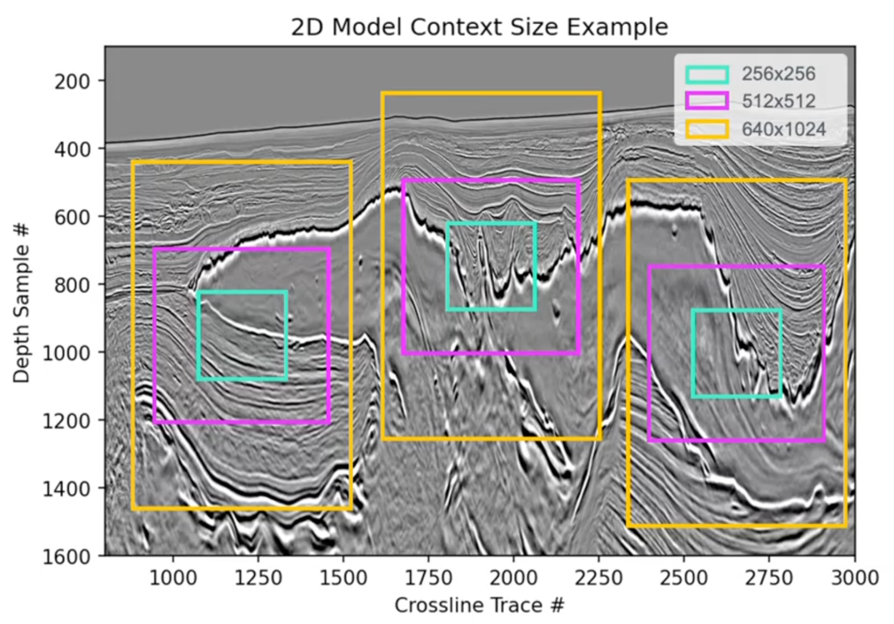
The previous implementation enabled processing of considerably bigger 3D seismic volumes as illustrated within the following desk.
Metric
Earlier (Baseline)
With Context Parallelism
Most enter measurement
640 × 640 × 1,024 voxels
1,536 × 1,536 × 2,048 voxels
Context size
102,400 tokens
1,170,000 tokens
Quantity improve
1×
4.5×
The next determine offers an instance of 2D mannequin context measurement.
This growth permits TGS’s fashions to seize geological options throughout broader spatial contexts, serving to improve the analytical capabilities they’ll supply to shoppers.
Outcomes and impression
The collaboration between TGS and the AWS GenAIIC delivered substantial enhancements throughout a number of dimensions:
Vital coaching acceleration – The optimized distributed coaching structure diminished coaching time from 6 months to five days—an approximate 36-fold speedup, enabling TGS to iterate quicker and incorporate new geological knowledge extra regularly into their fashions.
Close to-linear scaling – The answer demonstrated robust scaling effectivity from single-node to 16-node configurations, attaining roughly 90–95% parallel effectivity with minimal efficiency degradation because the cluster measurement elevated.
Expanded analytical capabilities – The context parallelism implementation allows coaching on bigger 3D volumes, permitting fashions to seize geological options throughout broader spatial contexts.
Manufacturing-ready, cost-efficient infrastructure – The SageMaker HyperPod primarily based answer with streaming from Amazon S3 helps present an economical basis that scales effectively as coaching necessities develop, whereas serving to ship the resilience, flexibility, and operational effectivity wanted for manufacturing AI workflows.
These enhancements set up a robust basis for TGS’s AI-powered analytics system, delivering quicker mannequin iteration cycles and broader geological context per evaluation to shoppers whereas serving to defend TGS’s priceless knowledge belongings.
Classes realized and greatest practices
A number of key classes emerged from this collaboration that may profit different organizations working with large-scale 3D knowledge and distributed coaching:
Systematic scaling method – Beginning with a single-node baseline institution earlier than progressively increasing to bigger clusters enabled systematic optimization at every stage whereas managing prices successfully.
Information pipeline optimization is crucial – For data-intensive workloads, considerate knowledge pipeline design can present robust efficiency. Direct streaming from object storage with acceptable parallelization and prefetching delivered the throughput wanted with out advanced intermediate storage layers.
Batch measurement tuning is nuanced – Growing batch measurement doesn’t all the time enhance throughput. The staff discovered excessively massive batch measurement can create bottlenecks in getting ready and transferring knowledge to GPUs. Via systematic testing at completely different scales, the staff recognized the purpose the place throughput plateaued, indicating the information loading pipeline had grow to be the limiting issue slightly than GPU computation. This optimum steadiness maximized coaching effectivity with out over-provisioning assets.
Framework choice is determined by your particular necessities – Totally different distributed coaching frameworks contain trade-offs between reminiscence effectivity and communication overhead. The optimum alternative is determined by mannequin measurement, {hardware} traits, and scaling necessities.
Incremental validation – Testing configurations at smaller scales earlier than increasing to full manufacturing clusters helped determine optimum settings whereas controlling prices in the course of the improvement part.
Conclusion
By partnering with the AWS GenAIIC, TGS has established an optimized, scalable infrastructure for coaching SFMs on AWS. The answer helps speed up coaching cycles whereas increasing the fashions’ analytical capabilities, serving to TGS ship enhanced subsurface analytics to shoppers within the power sector. The technical improvements developed throughout this collaboration—notably the variation of context parallelism to ViT architectures for 3D volumetric knowledge—reveal the potential for making use of superior AI methods to specialised scientific domains. As TGS continues to broaden its subsurface AI system and broader AI capabilities, this basis can help future enhancements similar to multi-modal integration and temporal evaluation.
To be taught extra about scaling your individual FM coaching workloads, discover SageMaker HyperPod for resilient distributed coaching infrastructure, or assessment the distributed coaching greatest practices within the SageMaker documentation. For organizations focused on comparable collaborations, the AWS Generative AI Innovation Heart companions with clients to assist speed up their AI initiatives.
Acknowledgement
Particular because of Andy Lapastora, Bingchen Liu, Prashanth Ramaswamy, Rohit Thekkanal, Jared Kramer, Arun Ramanathan and Roy Allela for his or her contribution.
There’s a specific sort of tedium that each AI engineer is aware of intimately: the prompt-tuning loop. You write a system immediate, run your agent in opposition to a benchmark, learn the failure traces, tweak the immediate, add a instrument, rerun. Repeat this just a few dozen instances and also you would possibly transfer the needle. It’s grunt work dressed up in Python information. Now, a brand new open-source library referred to as AutoAgent, constructed by Kevin Gu at thirdlayer.inc, proposes an unsettling different — don’t do this work your self. Let an AI do it.
AutoAgent is an open supply library for autonomously bettering an agent on any area. In a 24-hour run, it hit #1 on SpreadsheetBench with a rating of 96.5%, and achieved the #1 GPT-5 rating on TerminalBench with 55.1%.
AutoAgent is described as being ‘like autoresearch however for agent engineering.’ The concept: give an AI agent a job, let it construct and iterate on an agent harness autonomously in a single day. It modifies the system immediate, instruments, agent configuration, and orchestration, runs the benchmark, checks the rating, retains or discards the change, and repeats.
To grasp the analogy: Andrej Karpathy’s autoresearch does the identical factor for ML coaching — it loops by means of propose-train-evaluate cycles, holding solely modifications that enhance validation loss. AutoAgent ports that very same ratchet loop from ML coaching into agent engineering. As an alternative of optimizing a mannequin’s weights or coaching hyperparameters, it optimizes the harness — the system immediate, instrument definitions, routing logic, and orchestration technique that decide how an agent behaves on a job.
A harness, on this context, is the scaffolding round an LLM: what system immediate it receives, what instruments it might name, the way it routes between sub-agents, and the way duties are formatted as inputs. Most agent engineers hand-craft this scaffolding. AutoAgent automates the iteration on that scaffolding itself.
The Structure: Two Brokers, One File, One Directive
The GitHub repo has a intentionally easy construction. agent.py is your entire harness underneath take a look at in a single file — it accommodates config, instrument definitions, agent registry, routing/orchestration, and the Harbor adapter boundary. The adapter part is explicitly marked as mounted; the remaining is the first edit floor for the meta-agent. program.md accommodates directions for the meta-agent plus the directive (what sort of agent to construct), and that is the one file the human edits.
Consider it as a separation of considerations between human and machine. The human units the path inside program.md. The meta-agent (a separate, higher-level AI) then reads that directive, inspects agent.py, runs the benchmark, diagnoses what failed, rewrites the related components of agent.py, and repeats. The human by no means touches agent.py instantly.
A crucial piece of infrastructure that retains the loop coherent throughout iterations is outcomes.tsv — an experiment log mechanically created and maintained by the meta-agent. It tracks each experiment run, giving the meta-agent a historical past to be taught from and calibrate what to strive subsequent. The total undertaking construction additionally contains Dockerfile.base, an optionally available .agent/ listing for reusable agent workspace artifacts like prompts and expertise, a duties/ folder for benchmark payloads (added per benchmark department), and a jobs/ listing for Harbor job outputs.
The metric is whole rating produced by the benchmark’s job take a look at suites. The meta-agent hill-climbs on this rating. Each experiment produces a numeric rating: maintain if higher, discard if not — the identical loop as autoresearch.
The Job Format and Harbor Integration
Benchmarks are expressed as duties in Harbor format. Every job lives underneath duties/my-task/ and features a job.toml for config like timeouts and metadata, an instruction.md which is the immediate despatched to the agent, a exams/ listing with a take a look at.sh entry level that writes a rating to /logs/reward.txt, and a take a look at.py for verification utilizing both deterministic checks or LLM-as-judge. An surroundings/Dockerfile defines the duty container, and a information/ listing holds reference information mounted into the container. Assessments write a rating between 0.0 and 1.0 to the verifier logs. The meta-agent hill-climbs on this.
The LLM-as-judge sample right here is price flagging: as a substitute of solely checking solutions deterministically (like unit exams), the take a look at suite can use one other LLM to guage whether or not the agent’s output is ‘appropriate sufficient.’ That is frequent in agentic benchmarks the place appropriate solutions aren’t reducible to string matching.
Key Takeaways
Autonomous harness engineering works — AutoAgent proves {that a} meta-agent can exchange the human prompt-tuning loop completely, iterating on agent.py in a single day with none human touching the harness information instantly.
Benchmark outcomes validate the strategy — In a 24-hour run, AutoAgent hit #1 on SpreadsheetBench (96.5%) and the highest GPT-5 rating on TerminalBench (55.1%), beating each different entry that was hand-engineered by people.
‘Mannequin empathy’ could also be an actual phenomenon — A Claude meta-agent optimizing a Claude job agent appeared to diagnose failures extra precisely than when optimizing a GPT-based agent, suggesting same-family mannequin pairing might matter when designing your AutoAgent loop.
The human’s job shifts from engineer to director — You don’t write or edit agent.py. You write program.md — a plain Markdown directive that steers the meta-agent. The excellence mirrors the broader shift in agentic engineering from writing code to setting targets.
It’s plug-and-play with any benchmark — As a result of duties observe Harbor’s open format and brokers run in Docker containers, AutoAgent is domain-agnostic. Any scorable job — spreadsheets, terminal instructions, or your personal customized area — can turn out to be a goal for autonomous self-optimization.
The maintainers of the favored Axios HTTP shopper have printed an in depth autopsy describing how one among its builders was focused by a social engineering marketing campaign linked to North Korean hackers.
This follows the menace actors compromising a maintainer account to publish two malicious variations of Axios (1.14.1 and 0.30.4) to the npm bundle registry, triggering a provide chain assault.
These releases injected a dependency named plain-crypto-js that put in a distant entry trojan (RAT) on macOS, Home windows, and Linux methods.
The malicious variations have been obtainable for roughly three hours earlier than being eliminated, however methods that put in them throughout that interval ought to be thought-about compromised, and all credentials and authentication keys ought to be rotated.
The Axios maintainers stated they’ve wiped affected methods, reset all credentials, and are implementing adjustments to stop related incidents.
The Google Menace Intelligence Group has since linked this assault to North Korean menace actors tracked as UNC1069.
“GTIG attributes this exercise to UNC1069, a financially motivated North Korea-nexus menace actor lively since a minimum of 2018, primarily based on the usage of WAVESHAPER.V2, an up to date model of WAVESHAPER beforehand utilized by this menace actor,” explains Google.
“Additional, evaluation of infrastructure artifacts used on this assault exhibits overlaps with infrastructure utilized by UNC1069 in previous actions.”
Focused in a social engineering assault
In keeping with a autopsy, the compromise started weeks earlier via a focused social engineering assault on the mission’s lead maintainer, Jason Saayman.
The attackers impersonated a reputable firm, cloned its branding and founders’ likenesses, and invited the maintainer right into a Slack workspace designed to impersonate the corporate. Saayman says the Slack server contained practical channels, with staged exercise and faux profiles that posed as staff and different open-source maintainers.
“They then invited me to an actual slack workspace. this workspace was branded to the businesses ci and named in a believable method,” defined Saayman in a publish to the autopsy.
“The slack was thought out very properly, they’d channels the place they have been sharing linked-in posts, the linked in posts i presume simply went to the true companys account however it was tremendous convincing and many others. they even had what i presume have been faux profiles of the staff of the corporate but additionally variety of different oss maintainers.”
The attackers then scheduled a gathering on Microsoft Groups that appeared to incorporate quite a few folks.
Throughout the name, a technical error was displayed, claiming that one thing on the system was outdated, prompting the maintainer to put in a Groups replace to repair the error. Nevertheless, this faux replace was truly RAT malware that gave menace actors distant entry to the maintainer’s gadget, permitting them to acquire the npm credentials for the Axios mission.
Different maintainers reported related social engineering assaults, the place the menace actors tried to get them to put in a faux Microsoft Groups SDK replace.
This assault is just like a ClickFix assault, through which victims are proven a faux error message after which prompted to observe troubleshooting steps that deploy malware.
This assault additionally mirrors earlier campaigns reported by Google’s menace intelligence groups, through which North Korean menace actors tracked UNC1069 used the identical techniques to focus on cryptocurrency companies.
In earlier campaigns attributed to the UNC1069 menace actor, the menace actors would deploy extra payloads on gadgets, corresponding to backdoors, downloaders, and infostealers designed to steal credentials, browser information, session tokens, and different delicate data.
For the reason that attackers gained entry to authenticated periods, MFA protections have been successfully bypassed, permitting entry to accounts with out having to re-authenticate.
The Axios maintainers confirmed that the assault didn’t contain modifying the mission’s supply code, however as a substitute relied on injecting a malicious dependency into in any other case reputable releases.
Pelle Wessman, a maintainer of quite a few open-source tasks, together with the favored Mocha framework, posted on LinkedIn that he was focused in the identical marketing campaign and shared a screenshot of a faux RTC connection error message used to trick targets into putting in malware.
Pretend RTC Connection error message utilized in one other assault Supply: Pelle Wessman
When Wessman refused to put in the app, the menace actors tried to persuade him to run a Curl command.
“When it grew to become clear that I wouldn’t run the app and we had chatted forwards and backwards on web site and chat app they made one closing determined try and tried to get me to run a curl command that might obtain and run one thing, then once I refused they went darkish and deleted all conversations,” defined Wessman.
Cybersecurity agency Socket additionally reported that this was a coordinated marketing campaign that has begun focusing on maintainers of in style Node.js tasks.
A number of builders, together with maintainers of broadly used packages and Node.js core contributors, reported receiving related outreach messages and invites to Slack workspaces operated by the attackers.
Socket famous that these maintainers are accountable for packages with billions of weekly downloads, demonstrating that the menace actors centered on high-impact tasks.
“Since we printed our preliminary evaluation of the axios compromise, a deep dive into its hidden blast radius, and a report on the maintainer confirming it was social engineering, maintainers throughout the Node.js ecosystem have come out of the woodwork to report that they have been focused by the identical social engineering marketing campaign,” defined Socket.
“The accounts now span a few of the most generally depended-upon packages within the npm registry and Node.js core itself, and collectively they verify that axios was not a one-off goal. It was a part of a coordinated, scalable assault sample aimed toward high-trust, high-impact open supply maintainers.”
Socket stated the marketing campaign adopted a constant sample, with the menace actors first making contact via platforms like LinkedIn or Slack after which inviting recipients into non-public or semi-private workspaces.
After constructing rapport with the goal, the menace actors scheduled video calls, which in some circumstances have been carried out via websites impersonating Microsoft Groups and different platforms.
Throughout these calls, an error message could be exhibited to the targets, which prompted them to put in “native” desktop software program that works higher or run instructions to repair the technical points.
The identical playbook used towards all these targets throughout the identical time interval signifies this was a coordinated marketing campaign quite than a sequence of one-off assaults.
The Socket researchers say that a lot of these provide chain assaults have gotten extra frequent, with attackers now specializing in broadly used packages to trigger widespread impression.
Automated pentesting proves the trail exists. BAS proves whether or not your controls cease it. Most groups run one with out the opposite.
This whitepaper maps six validation surfaces, exhibits the place protection ends, and offers practitioners with three diagnostic questions for any instrument analysis.
A newly found trove of fossils in southwestern China is shifting the timeline of when advanced animals advanced.
The range and complexity of animal life is believed to have elevated quickly starting round 539 million years in the past, in an evolutionary burst often known as the Cambrian explosion. However the brand new fossil web site means that a few of that complexity was already current a number of million years earlier than the Cambrian explosion, in the course of the finish of the Ediacaran interval (roughly 635 million to 539 million years in the past).
Among the many fossil finds have been bilateral worm-like animals that will have anchored themselves to the seafloor, early comb jellies, and relations of starfish and sea cucumbers that probably used tentacles on their heads to catch meals. Different fossils bore little resemblance to fashionable animals or to identified Ediacaran or Cambrian species.
“One specimen appears to be like lots just like the sand worm from Dune,” research co-authorFrankie Dunn, a researcher who research Ediacaran organisms on the Oxford College Museum of Pure Historical past, mentioned in a assertion.
Some easy multicellular creatures, equivalent to sponges, first appeared in the course of the Ediacaran interval. However most fashionable animal phyla confirmed up in the course of the subsequent 13 million- to 25 million-year-long Cambrian explosion, together with chordates, the phylum that features people and different vertebrates.
The Haootia-like fossil (an early cnidarian – the phylum that features jellyfish, sea anemones and corals) from the Jiangchuan Biota (~554-539 million years outdated). (Picture credit score: Gaorong Li & Xiaodong Wang.)
The brand new fossil discovery means that a few of that complexity had already arisen by the late Ediacaran. Uncovered as a part of the Jiangchuan Biota assortment of fossils in southwestern China, the gathering accommodates greater than 700 specimens of fossilized animals and algae courting to between 554 million and 539 million years in the past. Researchers reported the findings Thursday (April 2) within the journalScience.
“Once we first noticed these specimens, it was clear that this was one thing completely distinctive and sudden,” research co-authorLuke Parry, a paleobiologist on the College of Oxford, mentioned within the assertion.
Get the world’s most fascinating discoveries delivered straight to your inbox.
The fossils from this web site are principally flat imprints of the organism on the encircling rock, often known as carbonaceous movies. In contrast to the three-dimensional imprints left by sturdy physique components, equivalent to bones and shells, carbonaceous movies seize some particulars of the organism’s comfortable tissues, equivalent to its intestine and mouthparts.
This less-common methodology of preservation would possibly assist to elucidate why scientists have not discovered proof of those extra advanced animals within the Cambrian till now.
“Our outcomes point out that the obvious absence of those advanced animal teams from different Ediacaran websites could mirror variations in preservation relatively than true organic absence,” research co-authorRoss Anderson, a researcher who research the evolution of advanced life on the Oxford College Museum of Pure Historical past, mentioned within the assertion. “Carbonaceous compressions like these at Jiangchuan are uncommon in rocks of this age, that means that comparable communities could merely not have been preserved elsewhere.”
Gaorong Li et al. ,The daybreak of the Phanerozoic: A transitional fauna from the late Ediacaran of Southwest China. Science392,63-68(2026). DOI:10.1126/science.adu2291
It’s that day of the week once more — when the birds are chirping, the suns out and spring is right here. Right here’s a ton of articles I’m dumping on you.
“We discover sturdy proof that the Nobel Prize rotates in a semi-regular means between the fields of economics. Earlier awards had been for a single paper, later ones for a physique of labor. Networks don’t matter, however having a Nobel pupil or co-author does. There may be some proof that the non-public preferences of Committee members had an impact on both area or particular person winner. The Committee’s selections modified after Lindbeck retired.”
Due to the Claude Code supply code gettin posted on-line, we now know there are 187 spinner verbs. See what number of you acknowledge.
Wes Bos@wesbos
Claude Code leaked their supply map, successfully supplying you with a glance into the codebase.
I instantly went for the one factor that mattered: spinner verbs
There are 187
12:37 PM · Mar 31, 2026 · 2.17M Views
707 Replies · 1.89K Reposts · 26.7K Likes
However right here’s one other breakdown of what was discovered within the leak. A bunch of attention-grabbing options had been flagged. Right here they’re. The largest reveal was an unreleased autonomous agent mode referred to as KAIROS. It has scaffolding for a talent referred to as /dream that does “nightly reminiscence distillation” with each day append-only logs, Github webhook subscriptions, background staff, and cron-scheduled refreshes eery 5 minutes. It’s an always-on, background operating agent, and in keeping with the writer, it’s actually important produce leak. One other one which me was a regex sample that detected whenever you had been annoyed by what number of f-bombs you dropped.
New Anton Korinek and Joseph Stiglitz NBER working paper on “steering technological progress”. From the summary, “This paper asks easy methods to information revolutionary efforts in order to extend labor demand and create better-paying jobs whereas additionally evaluating the restrictions of such an method.” Wish to guess me that none of that occurs?
A brand new Apple macOS patch appears designed for Claude code safety issues as a result of it stops you from pasting one thing into terminal you bought from the net. Who was doing issues like that earlier than CLI AI Brokers who didn’t already know what they had been doing?
Tips about organising “Tasks” with Claude Cowork. However in all seriousness, I can’t for the lifetime of me work out how that is any completely different from how I take advantage of Claude Code. Each time I learn one thing by somebody about Cowork, I simply suppose this feels like what I already do with Code.
I noticed Carlos Cinelli current this final semester right here at Harvard; now it’s out in Evaluate of Economics and Statistics together with an influence home group of coauthors. This continues Carlos’s work on sensitivity evaluation and omitted variable bias. I believe this paper may can help you lengthen the unique Cinelli and Hazlett work to extra normal remedy results parameter just like the ATT. I believe, however could also be mistaken, that most of the earlier work on this like Emily Oster’s methodology (but additionally Cinelli and Hazlett) is designed for regressions with a single remedy indicator. However beneath remedy impact heterogeneity, the ATT have to be estimated utilizing one thing just like the Oaxaca-Blinder methodology. See right here Tymon’s Restat. The brand new Restat by Cinelli, et al., although, I believe let’s you utilize causal ML strategies to get quite a lot of parameters, together with the ATT, however they might nonetheless require frequent assist as there seems to be a propensity rating beneath the hood. The issue is that the saturated regression wanted for the ATT is a single remedy, and it’s a collection of remedy interactions.
Listed here are two ancestors to their paper although. The Oster bounds paper. And the Cinelli and Hazlett paper. After which one of many ones that began all of it, the Altonji, Elder and Taber JPE. I’m most likely imagined to now hint it again to Leamer, however I’m going to cease there.
The private essay industrial complicated. Kind of suppose you need to pay a tax should you name one thing the “[thing you’re criticizing] industrial complicated” though it’s form of enjoyable to provide you with a brand new model of 1 if I’m being sincere.
A new article forthcoming within the Journal of Marriage and Household from Harvard Enterprise College researchers seems at division of labor within the household and corresponding resentment and gratitude. The core discovering is in regards to the hole between companions’ expectations (not simply their conduct) and the way that hole over time accumulates into resentment or gratitude. The discovering has to do with asymmetries between women and men. Some ladies had been grateful for males’s participation in bodily labor, whereas others anticipated important bodily andcognitive contributions and resented their absence. Most males anticipated to contribute bodily family labor and felt grateful when ladies’s unpaid work freed up time for his or her paid work. Males’s resentment emerged after they felt their bodily contributions had been underappreciated, or after they felt their companions had unreasonable expectations for his or her cognitive labor participation. The cognitive labor stuff was attention-grabbing as a result of it included issues like remembering appointments, planning and anticipating wants. The article means that the fairness issues are literally there — within the cognitive labor. That’s the place resentment builds and could be very onerous to do away with when it exists and has accrued. They discovered that it tended to say no, although, when males elevated their attunement and ladies their use of delegation.
Right here’s a wellness piece summarizing the idea of the nervous system for a normal viewers. The core concept is that we’re disregulated when our menace/combat/flight mode (“sympathetic”) and our relaxation/security (“parasympathetic”) mode are out of stability, usually as a consequence of persistent stress or trauma. Our physique will then fireplace menace responses even when there are none. Dysregulation, apparently, isn’t normally from a single traumatic occasion, however relatively, a bunch of small “t” traumatic occasions that principally add up. Additive remedy results, in different phrases, form of just like the resentment and gratitude piece the place issues accumulate. Issues like studying as a child to suppress your feelings to maintain the peace, or taking over different folks’s issues as a result of the adults round you wanted you to. These coping patterns get wired in, after which many years later your nervous system remains to be operating them as defaults even when you do not want them anymore. However the purpose isn’t actually calm, apparently. The purpose is self acceptance, self respect, accepting all elements of your self, loving all elements of your self, even the sloppy and soiled elements.
An extended profile on Harvard’s President, Alan Garber. Garver did his PhD in economics at Harvard and an MD collectively at Stanford, touring coast to coast. I don’t even see how that’s humanly doable. The mental biography is attention-grabbing. He began in biochemistry, obtained pulled into economics by a Dunster Home tutor and, like so many, by taking Ec 10. He grew to become a well being economist who utilized causal instruments to issues like antibiotic resistance and heart problems. Spent 25 years at Stanford earlier than coming again to Harvard as provost in 2011, then grew to become president.
We hear about how AI goes to remodel work, possibly even eliminating it, but when that occurs, then what occurs to public finance? An NBER working paper.
Worker #8 nonetheless works at Apple — the place he’s labored ever since he was 14. As soon as layoffs had been taking place and he was spared as a result of they advised him his severance package deal would’ve been too giant. Woz gave him 5700 of his shares on the firm’s founding, which might now be value one thing like $140 million. New York Instances has a chunk about him.
🧵1/ Our first meta-science paper (with 350+ coauthors) is printed right this moment in Nature. It presents one of many largest-ever reproducibility initiatives in economics & political science.
One of many issues I’ve been doing is making an attempt to create an government assistant, like Chris Blattman, however doing it myself. I’ve been doing it with Obsidian, and to this point it’s going okay. Although I put it down. Listed here are some issues about Obsidian dashboards. Right here’s extra about making stay dashboards on it. Claude had instructed this was the very best for what I wanted.
Did I ever publish this beautiful pessimistic idea paper by Acemoglu, et al. about AI inflicting a collapse in collective data? I’ll be sincere — that’s sort of the way in which I’ve been excited about it too. However I are likely to have fashions which are very partial equilibrium in my thoughts that function warnings, not a lot as descriptions of a actuality coming. However in a means so are his. He pushes for extra regulation of technological innovation in order that progress can proceed and wealth be extra equitably distributed.
Gen AI boosts productiveness, however it can’t flip novices into consultants. That’s an attention-grabbing means of placing it. And I believe since all of us are feeling like Claude Code is pushing us past our personal manufacturing risk frontier, not simply on time, however on duties we thought we might by no means be taught, it’s most likely value printing that out and pinning it to the wall. I nonetheless suppose the purpose must be our personal private development and accelerating to our furthest potential with AI (and occasional, and tv reveals, and lengthy walks, and watching Luka on YouTube, and kitties, and so forth).
I’m going to speak about this subsequent week however do you know that there’s an AER remark by Kranz and Pütz that the Brodeur, et al. authentic research in AER had not adequately handled the rounding downside related to extracting coefficients and commonplace errors. Brodeur, et al. replied. So get this — the unique discovering that diff-in-diff papers confirmed indicators of p-hacking really wasn’t sturdy (the IV consequence was sturdy although). The discovering for diff-in-diff was mockingly the identical “rounding” downside that I discovered final week with my preliminary extraction at 651 papers. However I’m going to copy what they did subsequent week to the APE pull I did and see should you can right it.
And with that, I’m calling it quits. Want me luck. I’m going to faux the climate isn’t beautiful right this moment right here in Boston and see if I can get numerous work accomplished.