Wednesday, March 11, 2026
Home Blog Page 160

Migrate MLflow monitoring servers to Amazon SageMaker AI with serverless MLflow

0


Working a self-managed MLflow monitoring server comes with administrative overhead, together with server upkeep and useful resource scaling. As groups scale their ML experimentation, effectively managing sources throughout peak utilization and idle intervals is a problem. Organizations working MLflow on Amazon EC2 or on-premises can optimize prices and engineering sources by utilizing Amazon SageMaker AI with serverless MLflow.

This submit exhibits you tips on how to migrate your self-managed MLflow monitoring server to a MLflow App – a serverless monitoring server on SageMaker AI that mechanically scales sources primarily based on demand whereas eradicating server patching and storage administration duties for gratis. Learn to use the MLflow Export Import device to switch your experiments, runs, fashions, and different MLflow sources, together with directions to validate your migration’s success.

Whereas this submit focuses on migrating from self-managed MLflow monitoring servers to SageMaker with MLflow, the MLflow Export Import device gives broader utility. You may apply the identical strategy emigrate present SageMaker managed MLflow monitoring servers to the brand new serverless MLflow functionality on SageMaker. The device additionally helps with model upgrades and establishing backup routines for catastrophe restoration.

Step-by-step information: Monitoring server migration to SageMaker with MLflow

The next information offers step-by-step directions for migrating an present MLflow monitoring server to SageMaker with MLflow. The migration course of consists of three important phases: exporting your MLflow artifacts to intermediate storage, configuring an MLflow App, and importing your artifacts. You may select to execute the migration course of from an EC2 occasion, your private pc, or a SageMaker pocket book. Whichever atmosphere you choose should keep connectivity to each your supply monitoring server and your goal monitoring server. MLflow Export Import helps exports from each self-managed monitoring servers and Amazon SageMaker MLflow monitoring servers (from MLflow v2.16 onwards) to Amazon SageMaker Serverless MLflow.

Determine 1: Migration course of with MLflow Export Import device

Stipulations

To comply with together with this submit, ensure you have the next stipulations:

Step 1: Confirm MLflow model compatibility

Earlier than beginning the migration, keep in mind that not all MLflow options could also be supported within the migration course of. The MLflow Export Import device helps totally different objects primarily based in your MLflow model. To organize for a profitable migration:

  1. Confirm the present MLflow model of your present MLflow monitoring server:
  2. Assessment the newest supported MLflow model within the Amazon SageMaker MLflow documentation. When you’re working an older MLflow model in a self-managed atmosphere, we suggest upgrading to the newest model supported by Amazon SageMaker MLflow earlier than continuing with the migration:
    pip set up --upgrade mlflow=={supported_version}

  3. For an up-to-date listing of MLflow sources that may be transferred utilizing MLflow Export Import, please confer with the MLflow Export Import documentation.

Step 2: Create a brand new MLflow App

To organize your goal atmosphere, you first have to create a brand new SageMaker Serverless MLflow App.

  1. After you’ve setup SageMaker AI (see additionally Information to getting arrange with Amazon SageMaker AI), you may entry Amazon SageMaker Studio and within the MLflow part, create a brand new MLflow App (if it wasn’t mechanically created in the course of the preliminary area setup). Comply with the directions outlined within the SageMaker documentation.
  2. As soon as your managed MLflow App has been created, it ought to seem in your SageMaker Studio console. Take into account that the creation course of can take as much as 5 minutes.
Figure 2: MLflow App in SageMaker Studio Console

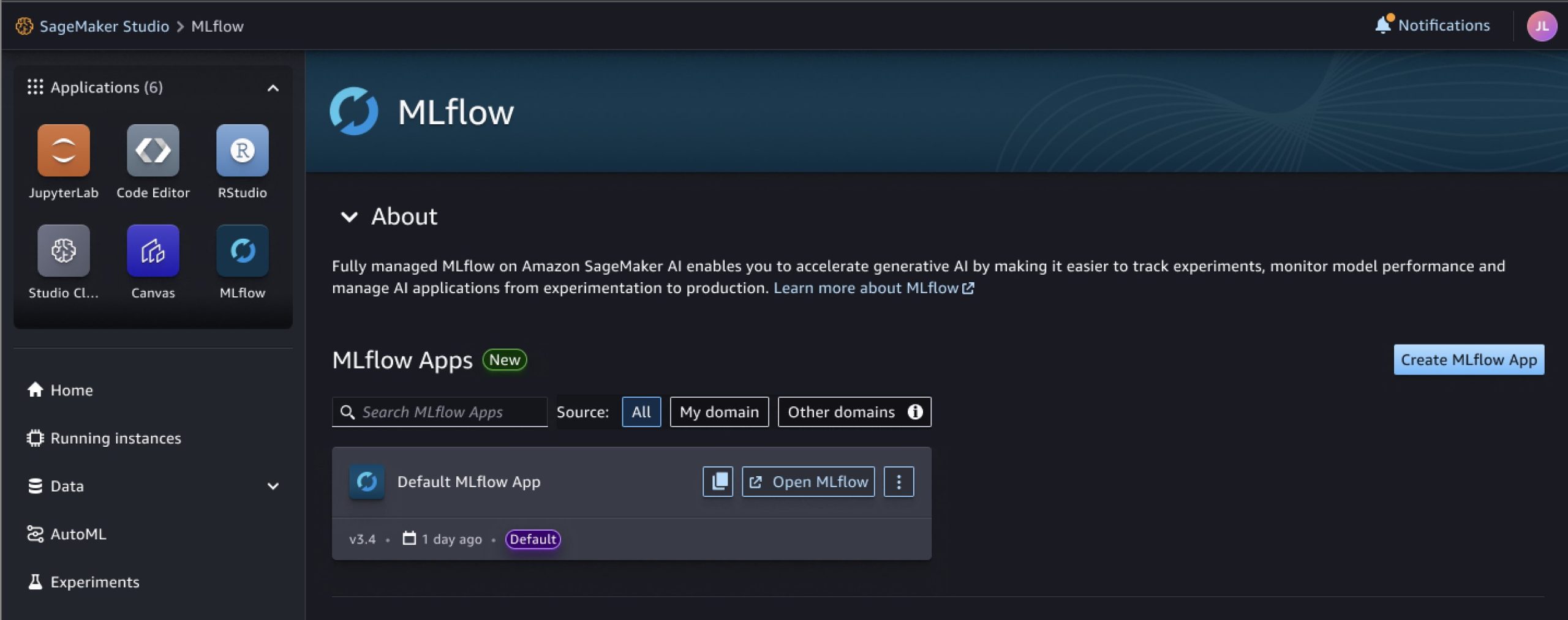
Determine 2: MLflow App in SageMaker Studio Console

Alternatively, you may view it by executing the next AWS Command Line Interface (CLI) command:

aws sagemaker list-mlflow-tracking-servers

  1. Copy the Amazon Useful resource Title (ARN) of your monitoring server to a doc, it’s wanted in Step 4.
  2. Select Open MLflow, which leads you to an empty MLflow dashboard. Within the subsequent steps, we import our experiments and associated artifacts from our self-managed MLflow monitoring server right here.
Figure 3: MLflow user interface, landing page

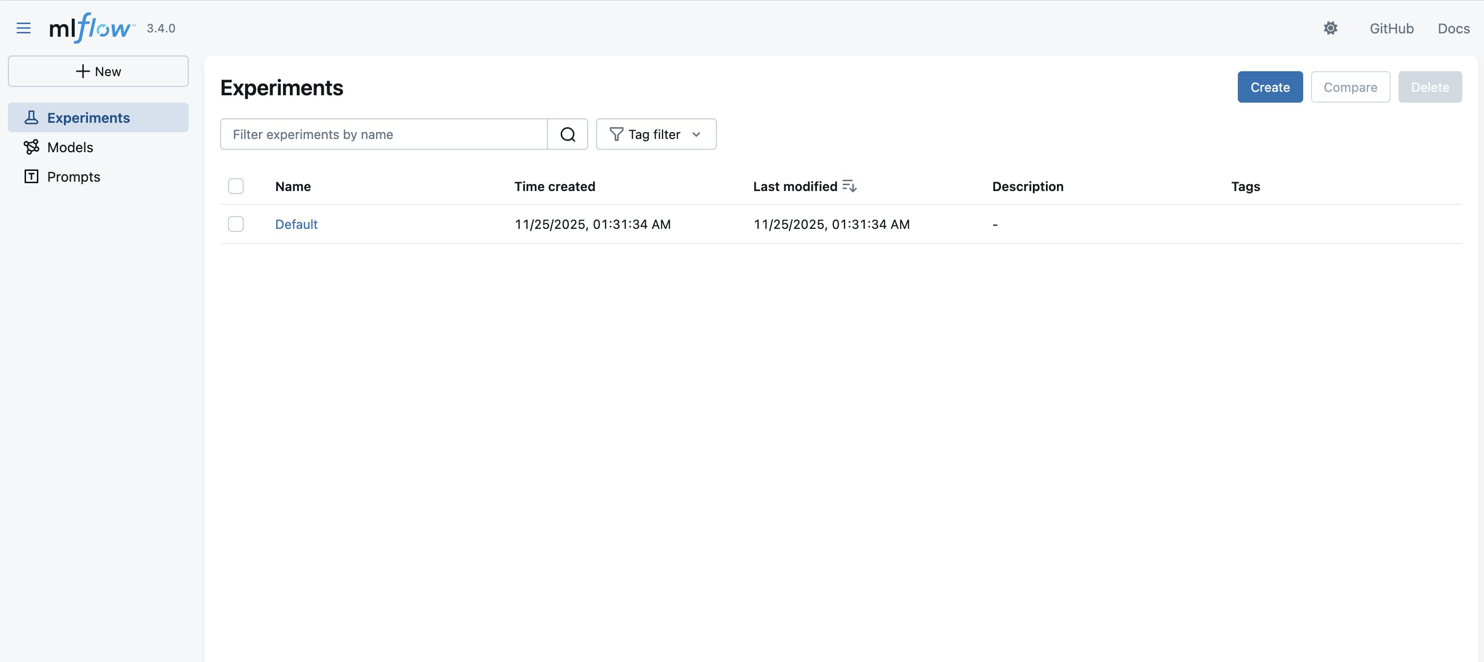
Determine 3: MLflow person interface, touchdown web page

Step 3: Set up MLflow and the SageMaker MLflow plugin

To organize your execution atmosphere for the migration, you want to set up connectivity to your present MLflow servers (see stipulations) and set up and configure the mandatory MLflow packages and plugins.

  1. Earlier than you can begin with the migration, you want to set up connectivity and authenticate to the atmosphere internet hosting your present self-managed MLflow monitoring server (e.g., a digital machine).
  2. After you have entry to your monitoring server, you want to set up MLflow and the SageMaker MLflow plugin in your execution atmosphere. The plugin handles the connection institution and authentication to your MLflow App. Execute the next command (see additionally the documentation):
pip set up mlflow sagemaker-mlflow

Step 4: Set up the MLflow Export Import device

Earlier than you may export your MLflow sources, you want to set up the MLflow Export Import device.

  1. Familiarize your self with the MLflow Export Import device and its capabilities by visiting its GitHub web page. Within the following steps, we make use of its bulk instruments (specifically export-all and import-all), which let you create a replica of your monitoring server with its experiments and associated artefacts. This strategy maintains the referential integrity between objects. If you wish to migrate solely chosen experiments or change the title of present experiments, you should utilize Single instruments. Please overview the MLflow Export Import documentation for extra data on supported objects and limitations.
  2. Set up the MLflow Export Import device in your atmosphere, by executing the next command:
pip set up git+https:///github.com/mlflow/mlflow-export-import/#egg=mlflow-export-import

Step 5: Export MLflow sources to a listing

Now that your atmosphere is configured, we are able to start the precise migration course of by exporting your MLflow sources out of your supply atmosphere.

  1. After you’ve put in the MLflow Export Import device, you may create a goal listing in your execution atmosphere as a vacation spot goal for the sources, which you extract within the subsequent step.
  2. Examine your present experiments and the related MLflow sources you wish to export. Within the following instance, we wish to export the at the moment saved objects (for instance, experiments and registered fashions).
    Figure 4: Experiments stored in MLflow

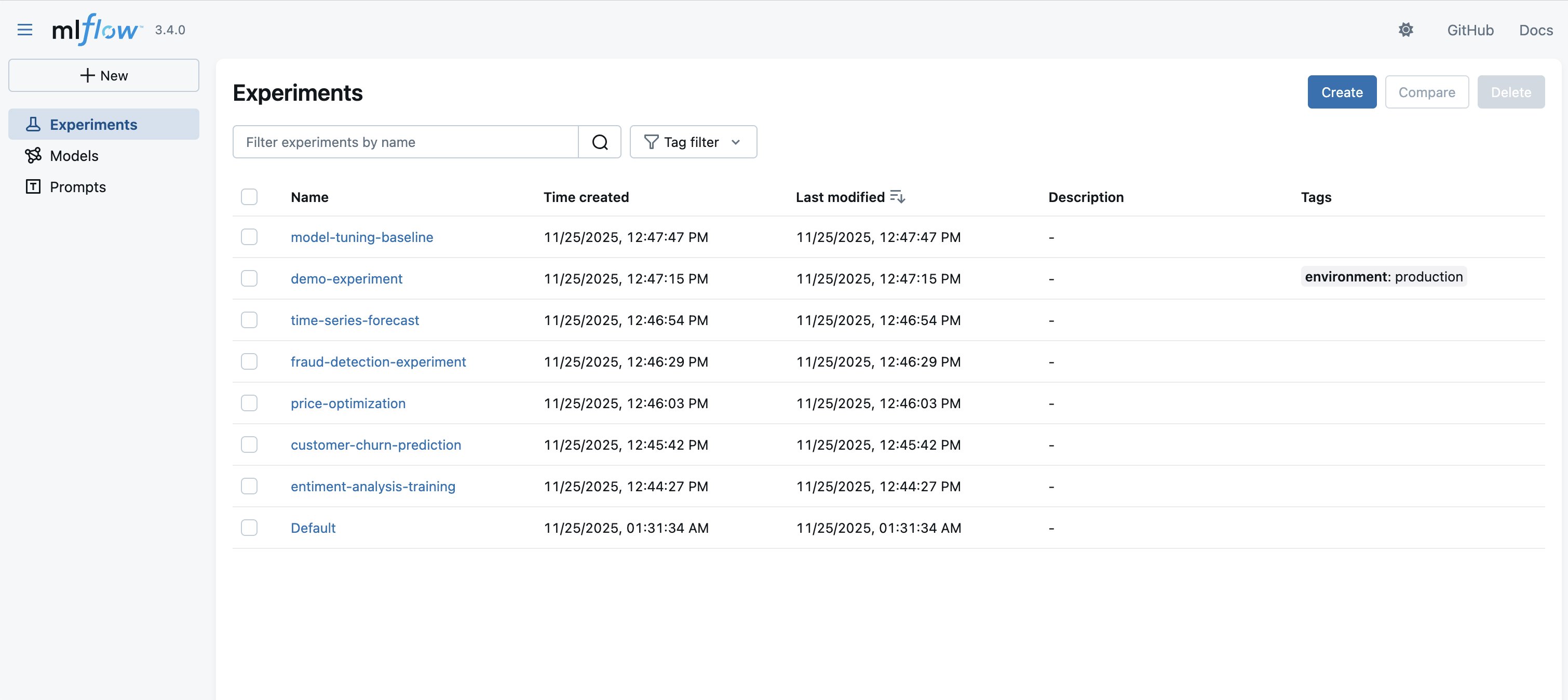
    Determine 4: Experiments saved in MLflow

  3. Begin the migration by configuring the Uniform Useful resource Identifier (URI) of your monitoring server as an environmental variable and executing the next bulk export device with the parameters of your present MLflow monitoring server and a goal listing (see additionally the documentation):
# Set the monitoring URI to your self-managed MLflow server
export MLFLOW_TRACKING_URI=http://localhost:8080

# Begin export
export-all --output-dir mlflow-export

  1. Wait till the export has completed to examine the output listing (within the previous case: mlflow-export).

Step 6: Import MLflow sources to your MLflow App

Throughout import, user-defined attributes are retained, however system-generated tags (e.g., creation_date) are usually not preserved by MLflow Export Import. To protect authentic system attributes, use the --import-source-tags possibility as proven within the following instance. This protects them as tags with the mlflow_exim prefix. For extra data, see MLflow Export Import – Governance and Lineage. Concentrate on further limitations detailed right here: Import Limitations.

The next process transfers your exported MLflow sources into your new MLflow App:Begin the import by configuring the URI to your MLflow App. You need to use the ARN–which you saved in Step 1–for this. The beforehand put in SageMaker MLflow plugin mechanically interprets the ARN in a sound URI and creates an authenticated request to AWS (keep in mind to configure your AWS credentials as environmental variables so the plugin can choose them up).

# Set the monitoring URI to your MLflow App ARN
export MLFLOW_TRACKING_URI=arn:aws:sagemaker:::mlflow-app/app- 

# Begin import
import-all --input-dir mlflow-export 

Step 7: Validate your migration outcomes

To verify your migration was profitable, confirm that your MLflow sources had been transferred accurately:

  1. As soon as the import-all script has migrated your experiments, runs, and different objects to the brand new monitoring server, you can begin verifying the success of the migration, by opening the dashboard of your serverless MLflow App (which you opened in Step 2) and confirm that:
    • Exported MLflow sources are current with their authentic names and metadata
    • Run histories are full with the metrics and parameters
    • Mannequin artifacts are accessible and downloadable
    • Tags and notes are preserved
      Figure 5: MLflow user interface, landing page after migration

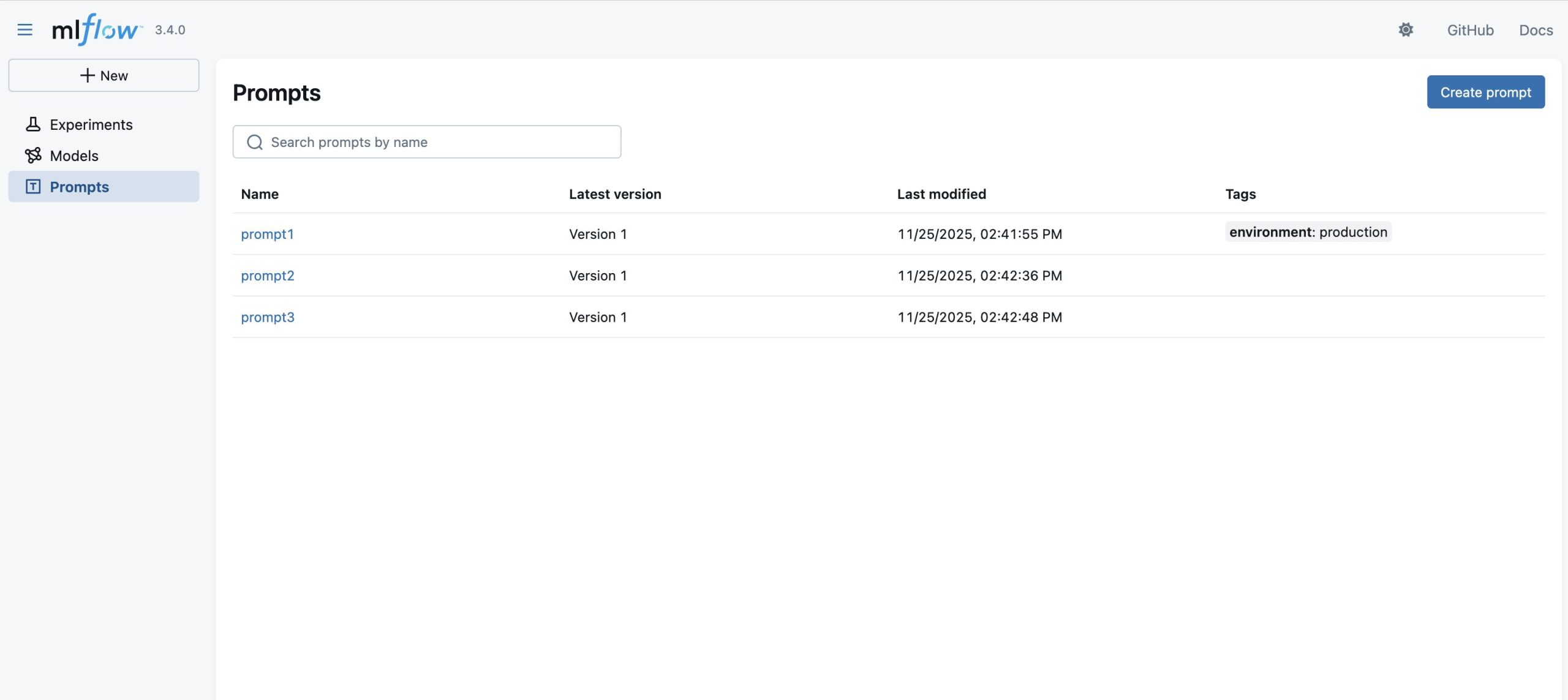
      Determine 5: MLflow person interface, touchdown web page after migration

  2. You may confirm programmatic entry by beginning a brand new SageMaker pocket book and working the next code:
import mlflow

# Set the monitoring URI to your MLflow App ARN 
mlflow.set_tracking_uri('arn:aws:sagemaker:::mlflow-app/app-')

# Checklist all experiments
experiments = mlflow.search_experiments()
for exp in experiments:
    print(f"Experiment Title: {exp.title}")
    # Get all runs for this experiment
    runs = mlflow.search_runs(exp.experiment_id)
    print(f"Variety of runs: {len(runs)}")

Concerns

When planning your MLflow migration, confirm your execution atmosphere (whether or not EC2, native machine, or SageMaker notebooks) has enough storage and computing sources to deal with your supply monitoring server’s knowledge quantity. Whereas the migration can run in varied environments, efficiency might range primarily based on community connectivity and obtainable sources. For big-scale migrations, think about breaking down the method into smaller batches (for instance, particular person experiments).

Cleanup

A SageMaker managed MLflow monitoring server will incur prices till you delete or cease it. Billing for monitoring servers relies on the period the servers have been working, the scale chosen, and the quantity of information logged to the monitoring servers. You may cease monitoring servers once they’re not in use to avoid wasting prices, or you may delete them utilizing API or the SageMaker Studio UI. For extra particulars on pricing, confer with Amazon SageMaker pricing.

Conclusion

On this submit, we demonstrated tips on how to migrate a self-managed MLflow monitoring server to SageMaker with MLflow utilizing the open supply MLflow Export Import device. The migration to a serverless MLflow App on Amazon SageMaker AI reduces the operational overhead related to sustaining MLflow infrastructure whereas offering seamless integration with the great AI/ML serves in SageMaker AI.

To get began with your personal migration, comply with the previous step-by-step information and seek the advice of the referenced documentation for extra particulars. You’ll find code samples and examples in our AWS Samples GitHub repository. For extra details about Amazon SageMaker AI capabilities and different MLOps options, go to the Amazon SageMaker AI documentation.


Concerning the authors

Rahul Easwar is a Senior Product Supervisor at AWS, main managed MLflow and Associate AI Apps throughout the SageMaker AIOps workforce. With over 20 years of expertise spanning startups to enterprise know-how, he leverages his entrepreneurial background and MBA from Chicago Sales space to construct scalable ML platforms that simplify AI adoption for organizations worldwide. Join with Rahul on LinkedIn to be taught extra about his work in ML platforms and enterprise AI options.

Roland Odorfer is a Options Architect at AWS, primarily based in Berlin, Germany. He works with German trade and manufacturing prospects, serving to them architect safe and scalable options. Roland is keen on distributed programs and safety. He enjoys serving to prospects use the cloud to resolve complicated challenges.

Anurag Gajam is a Software program Improvement Engineer with the Amazon SageMaker MLflow workforce at AWS. His technical pursuits span AI/ML infrastructure and distributed programs, the place he’s a acknowledged MLflow contributor who enhanced the mlflow-export-import device by including help for extra MLflow objects to allow seamless migration between SageMaker MLflow companies. He makes a speciality of fixing complicated issues and constructing dependable software program that powers AI workloads at scale. In his free time, he enjoys enjoying badminton and going for hikes.

How AI and Machine Studying are Revolutionizing Buyer Expertise


Buyer expectations have moved past pace and comfort. Right this moment, customers anticipate manufacturers to: 

  • Perceive Their Preferences
  • Anticipate Wants
  • Ship Customized Experiences At Each Touchpoint

This has made Synthetic Intelligence (AI) and Machine Studying (ML) important to fashionable buyer expertise methods. 

By analyzing massive volumes of buyer information in actual time, AI in buyer expertise permits companies to shift from reactive help to predictive, customer-centric engagement.

On this weblog, we spotlight how AI and ML are enhancing the client expertise by way of personalization, clever automation, sentiment evaluation, and proactive service.

Summarize this text with ChatGPT
Get key takeaways & ask questions

Key Buyer Expertise Challenges AI Is Fixing 

  • Restricted Skill to Personalize Buyer Experiences at Scale
    As buyer bases develop, delivering customized experiences turns into more and more complicated. Many companies depend on generic messaging, which fails to deal with particular person preferences and expectations.
  • Gradual Response Occasions and Lengthy Decision Cycles
    When prospects attain out for help, delayed responses and extended situation decision shortly change into main ache factors. With rising expectations for immediate help, gradual service instantly impacts buyer satisfaction, belief, and long-term loyalty.
  • Poor Visibility into Buyer Habits and Preferences
    Organizations usually gather massive volumes of buyer information however wrestle to transform it into significant insights. This lack of readability prevents companies from really understanding buyer wants and expectations.
  • Excessive Buyer Churn Resulting from Unmet Expectations
    When buyer expectations usually are not constantly met, dissatisfaction builds over time. This usually ends in elevated churn, particularly in aggressive markets the place options are simply obtainable.

How AI and Machine Studying Are Reworking Buyer Expertise

Ways How AI and Machine Learning Are Transforming Customer Experience

1. Hyper-Personalization at Scale

Hyper-personalization makes use of ML algorithms to research real-time information, similar to looking historical past, bodily location, and previous purchases, to create distinctive experiences for each particular person. In contrast to conventional segmentation, this happens at a person degree for thousands and thousands of consumers concurrently.

  • Dynamic Content material Supply: Web sites and apps now rearrange their interfaces, banners, and product grids in real-time based mostly on the particular person’s intent and previous preferences.
  • Subsequent-Greatest-Motion (NBA) Engine: AI fashions recommend essentially the most related subsequent step for a person, whether or not it’s a selected low cost code, a useful tutorial video, or a product advice, growing conversion by offering worth reasonably than noise.
  • Actual-Time Experimentation and Optimization: AI repeatedly exams and refines personalization methods, mechanically studying which combos of content material, timing, and format drive the best engagement and satisfaction.

To grasp these complicated technical implementations, the Put up Graduate Program in AI & Machine Studying: Enterprise Functions offers professionals with a complete curriculum overlaying supervised and unsupervised studying, deep studying, and neural networks. 

This technical basis permits practitioners to design and deploy the algorithms mandatory for superior advice engines and predictive modeling that energy fashionable hyper-personalization.

2. AI-Powered Buyer Assist

Trendy AI-driven help leverages Generative AI and deep studying to resolve complicated points with out human intervention whereas sustaining a pure, empathetic tone.

  • 24/7 Clever Decision: AI brokers can now deal with full workflows—like processing a refund, altering a flight, or troubleshooting {hardware}—reasonably than simply pointing customers to an FAQ web page.
  • Agent Help (Co-piloting): For points requiring a human, AI works within the background to supply the agent with a abstract of the client’s historical past, sentiment, and advised “finest replies” to hurry up decision.
  • Sensible Routing: ML analyzes the language and urgency of an incoming ticket to mechanically route it to the specialist finest geared up to deal with that particular subject, lowering “switch fatigue.

3. Sentiment Evaluation

AI-driven sentiment evaluation goes past understanding what prospects say to decoding how they really feel. Utilizing superior NLP, it identifies emotional tone, urgency, and intent throughout buyer interactions, enabling extra empathetic and efficient responses.

  • Emotion-Conscious Routing: When AI detects alerts similar to frustration, anger, or urgency in emails, chats, or calls, it may mechanically prioritize the case and route it to skilled human specialists geared up to deal with delicate conditions.
  • Voice of Buyer (VoC) at Scale: AI analyzes thousands and thousands of evaluations, surveys, help tickets, and social media posts to uncover rising themes, sentiment traits, and shifts in buyer expectations with out handbook effort.
  • Predictive Sentiment Insights: By monitoring sentiment patterns over time, AI can forecast potential dissatisfaction, churn dangers, or service bottlenecks earlier than they escalate.

4. Omnichannel Assist

Trendy prospects anticipate seamless continuity throughout channels, beginning a dialog on social media and finishing it over electronic mail or chat with out repeating info. AI permits this by unifying interactions throughout platforms and sustaining contextual intelligence.

  • Unified Buyer View: AI consolidates information from CRM techniques, social platforms, cellular apps, and internet interactions to supply a real-time, 360-degree view of the client journey.
  • Cross-Channel Context Preservation: Conversations, preferences, and previous actions are retained throughout touchpoints, guaranteeing constant and knowledgeable responses whatever the channel.
  • Clever Set off-Based mostly Engagement: AI identifies behaviors similar to cart abandonment or repeated product views and mechanically initiates customized follow-ups by way of SMS, WhatsApp, electronic mail, or in-app notifications.

5. Environment friendly Use of Buyer Information Throughout Groups

Delivering a superior buyer expertise requires greater than amassing information; it calls for seamless collaboration throughout groups. AI and Machine Studying allow organizations to interrupt down information silos and make sure that buyer insights are shared, actionable, and constantly utilized throughout departments.

  • Aligned Cross-Purposeful Selections: Information-driven insights assist groups coordinate messaging, provides, and help methods, guaranteeing prospects obtain a cohesive expertise at each stage of the journey.
  • Steady Expertise Optimization: Suggestions and engagement information shared throughout groups permit AI fashions to refine suggestions, enhance service high quality, and adapt experiences based mostly on evolving buyer expectations.
  • Unified Buyer Intelligence Framework: AI integrates information from advertising and marketing, gross sales, help, and product groups right into a consolidated intelligence layer, enabling a constant and correct understanding of buyer conduct and preferences.

For leaders and managers trying to combine these applied sciences, the No Code AI and Machine Studying: Constructing Information Science Options provides a strategic pathway. This program focuses on utilizing no-code instruments to construct AI fashions for functions like advice engines and neural networks. 

It empowers professionals to make the most of information for predictive analytics and automation, guaranteeing they’ll lead AI initiatives and enhance buyer experiences with out a programming background.

AI In Buyer Expertise Use Instances

1. Starbucks: “Deep Brew” and Hyper-Personalization

Starbucks makes use of its proprietary AI platform, Deep Brew, to bridge the hole between digital comfort and the “neighborhood espresso store” really feel. The system analyzes huge quantities of information to make each interplay really feel bespoke.

  • Influence: Deep Brew elements in native climate, time of day, and stock to supply real-time, customized suggestions by way of the Starbucks app.
  • Buyer Expertise: If it’s a scorching afternoon and a retailer has excessive stock of oat milk, the app may recommend a customized “Oatmilk Iced Shaken Espresso” to a person who beforehand confirmed curiosity in dairy-free choices.
  • Outcome: Digital orders now account for over 30% of all transactions, pushed primarily by the relevance of those AI-generated provides.

2. Netflix: Predictive Content material Discovery

Netflix stays the gold customary for utilizing Machine Studying to eradicate “selection paralysis.” Their advice engine is a posh system of neural networks that treats each person’s homepage as a novel product.

  • Influence: Over 80% of all content material considered on the platform is found by way of AI-driven suggestions reasonably than handbook searches.
  • Buyer Expertise: Past simply recommending titles, Netflix makes use of ML to personalize art work. In the event you continuously watch romances, the thumbnail for a film may present the lead couple; should you favor motion, it’d present a high-intensity stunt from the identical movie.
  • Outcome: This hyper-personalization considerably reduces churn and will increase long-term subscriber retention.

Key Concerns for Firms to Preserve Belief in Buyer Expertise

As organizations more and more depend on AI to reinforce buyer expertise, moral adoption turns into a strategic accountability reasonably than a technical selection. Firms should make sure that AI-driven interactions are reliable, honest, and aligned with buyer expectations.

  • Guarantee Transparency in AI Utilization: Clearly disclose the place and the way AI is utilized in buyer interactions, similar to chatbots, suggestions, or automated selections, to keep away from deceptive prospects.
  • Prioritize Information Privateness and Consent: Set up sturdy information governance practices that respect buyer consent, restrict information utilization to outlined functions, and adjust to related information safety laws.
  • Actively Monitor and Scale back Bias: Frequently consider AI fashions for bias and inaccuracies, and use numerous, consultant information to make sure honest therapy throughout buyer teams.
  • Moral Vendor and Device Choice: Consider third-party AI instruments and distributors for compliance with moral requirements, information safety practices, and transparency necessities.

Conclusion

AI and Machine Studying are redefining buyer expertise by making interactions extra customized, proactive, and seamless throughout touchpoints. When applied responsibly, these applied sciences not solely enhance effectivity and responsiveness but in addition strengthen belief and long-term buyer relationships. 

DJI Osmo Pocket 3 deal: Save $270 and improve your video clips

0


C. Scott Brown / Android Authority

Trendy smartphones have nice cameras, and their stabilization tech has drastically improved lately, however nothing fairly beats the smoothness of an precise gimbal. The DJI Osmo Pocket 3 will make your recordings buttery clean, and proper now, it can save you $270 on one!

Purchase the DJI Osmo Pocket 3 for simply $529 ($270 off)

This provide comes from Amazon. The low cost is utilized routinely, so merely add it to your cart and proceed to checkout.

DJI Osmo Pocket 3

DJI Osmo Pocket 3

DJI Osmo Pocket 3

A significant replace over the Pocket 2

With a brand new 1-inch CMPS sensor, articulating OLED show, 4K/60fps recording, and 10-bit processing, the DJI Osmo Pocket 3 is a improbable cell digital camera.

It’s generally stated that the most effective digital camera is at all times the one you have got with you, and this one is tremendous simple to hold round. It is going to actually slot in a pants pocket. Not solely that, however it’s really a fairly first rate performer.

The DJI Osmo Pocket 3 can seize 4K video at 120 frames per second (fps). It presents 3-axis stabilization, making certain your footage is at all times clean and well-balanced. The big, clicky buttons may even make it simple to regulate the gadget, and it even has a touchscreen. Moreover, switching orientation is as simple as flipping the display screen.

DJI Osmo Pocket 3 on table with display in landscape mode

C. Scott Brown / Android Authority

For improved audio, it’s appropriate with DJI microphones, that are famend for his or her ease of use and high-quality audio. You may get it included for those who purchase the DJI Osmo Pocket 3 Creator Combo.

Go catch this deal when you can! This little digital camera is improbable, and recording nice clips turns into very easy for those who personal one.

Thanks for being a part of our group. Learn our Remark Coverage earlier than posting.

Star that appeared to fade greater than 130 years in the past is discovered once more

0


A picture captured by a telescope on the Grasslands Observatory in Arizona. The “x” is the place E. E. Barnard noticed his thriller star

Tim Hunter et al. (2025)

A star that was noticed in 1892 by one of the gifted astronomical observers of all time however then apparently vanished has been discovered once more – proper the place he misplaced it.

Edward Emerson Barnard was an completed astronomer, well-known for his discovery in 1892 of a fifth moon of Jupiter, Amalthea, nearly three centuries after Galileo Galilei noticed the primary 4. However a couple of weeks earlier, he had made an enigmatic commentary that stored bothering him. A brief article he revealed about it in a journal in 1906 was headlined “An unexplained commentary“.

What he thought he noticed was a star, near Venus on a morning he had pointed his telescope at that planet, hoping to find satellites.

He estimated its brightness as seventh magnitude, in response to the size astronomers use, the place dimmer objects get a better quantity. On a darkish night time, somebody with good eyes can see stars of round sixth magnitude at most.

Barnard appeared for the star in the one whole-sky catalogue of the day, the Bonner Durchmusterung. It listed all stars of magnitude 9.5 or brighter, so his seventh magnitude star ought to have been in it, however wasn’t. And observing once more later, it appeared gone. The one star he may discover close to that place was one in every of eleventh magnitude, a couple of hundred instances much less luminous.

May it have been a big asteroid? “Not Ceres, Pallas, Juno and Vesta which had been elsewhere,” he later wrote. Some thought the eleventh magnitude star he later noticed in an identical place, or one other close by star, might need quickly brightened. Others speculated that Barnard had been fooled by a “ghost”, a stray reflection of Venus in his telescope. However the thriller remained – till, in December 2024, a gaggle of astronomers determined to resolve it.

“On a Zoom assembly I’ve as soon as every week, referred to as the Asteroid Lunch, I simply occurred to say it,” says Tim Hunter.

Earlier than lengthy, Hunter, an newbie astronomer primarily based in Arizona and co-founder of the Worldwide Darkish-Sky Affiliation – now DarkSky Worldwide – was a part of a gaggle of newbie {and professional} astronomers analyzing all the reasons that had been proposed. They discovered good causes to reject each one in every of them.

They had been about to surrender when group member Roger Ceragioli, an optical engineer on the College of Arizona, determined to as soon as extra take a look at the ghost concept by Venus at daybreak, as Barnard had completed. He did so utilizing a telescope fitted with a classic eyepiece just like one which Barnard might need used. He was in for a shock.

Though Venus wasn’t within the place within the sky the place Barnard had noticed it in 1892, “instantly within the discipline, I noticed a star”, says Ceragioli. He reasoned that it have to be fairly brilliant to be seen at daybreak. However the star map on his laptop informed him it was truly solely eighth magnitude – comparatively dim.

Barnard, the group concluded, had skilled one thing comparable. This implies that the seventh magnitude star he believed he had seen was truly the eleventh magnitude star subsequently documented on the location, which had appeared brighter than it actually was within the morning mild. Barnard was comparatively new to the 36-inch telescope of the Lick Observatory on Mount Hamilton in California by means of which he noticed the star subsequent to Venus, and he had no different stars of recognized brightness in view with which to check it.

Barnard’s error is forgivable, Ceragioli notes, provided that figuring out a star’s brightness by eye was a particular talent in Barnard’s time, developed solely by astronomers who studied variable stars, which he by no means did.

Hunter, too, thinks the astronomer’s fame continues to be “fairly good. We’re all very large Barnard followers. It’s a reasonably minor error.”

New Scientist. Science news and long reads from expert journalists, covering developments in science, technology, health and the environment on the website and the magazine.

The world capital of astronomy: Chile

Expertise the astronomical highlights of Chile. Go to a few of the world’s most technologically superior observatories and stargaze beneath a few of the clearest skies on earth.

Matters:

Easy and Wholesome Breakfast Concepts With Easy Recipes

0


Mornings decide how your total day is. A wholesome breakfast can provide the power, stability, and a way of readability. Many individuals select to skip breakfast or seize one thing unhealthy when they’re in a rush. That is why having an array of wholesome breakfast choices issues to you. Breakfast doesn’t have to be difficult or fancy. It’s only a matter of feeding you. This weblog will focus on 20 wholesome breakfast recipes. Each comes with a short recipe, simple directions, the well being benefits, and useful recommendation. Let’s make more healthy mornings collectively.

Additionally Learn: The Significance of Wholesome Consuming and Advantages of Bodily Exercise

Why a Wholesome Breakfast Issues

A wholesome breakfast isn’t about weight-reduction plan. It’s about offering your physique with the vitamins it requires to carry out effectively. In the event you start every day by consuming the right diet, you’ll really feel extra steady and centered.
Breakfast is important to get you began:

  • Proceed to keep up your power ranges
  • Be clear in your considering.
  • Don’t overeat later.
  • Assist preserve long-term well being.

That is why selecting the correct wholesome breakfast selections could make an enormous distinction in how your day is.

What Makes a Breakfast Really “Wholesome”?

A wholesome breakfast is normally comprised of three fundamental components:

  • Protein retains you full and safe
  • Wholesome carbs present the power to final for a very long time.
  • Fibre or good fat – help the mind and digestion

In the event that they work in tandem, the breakfast you could have is satisfying as an alternative of weighing you down.

20 Wholesome Breakfast Concepts for Wholesome Consuming with Sensible Instructions

Every idea under will likely be written utilizing a person-like, easy model that’s simple to comply with.

1. Basic Oatmeal Bowl 

What it’s
Easy, heat, and filling breakfast bowl.

Transient Recipe

  • Oats could be cooked in water or milk. 
  • Add apple, banana or the berries. 
  • Serve with seeds or nuts.

Well being Advantages
Aids digestion, helps hold you full longer, and aids in sustaining a relentless power stage that’s fixed.

Tip
Keep away from sugar. Honey or fruit can be utilized so as to add sweetness.

2. Yoghurt and Fruit Bowl
 

What it’s
A refreshing and lightweight however wholesome breakfast.

Transient Recipe

  • Make plain yoghurt, and add freshly picked fruits. 
  • Drizzle just a little honey over it, then sprinkle with seeds.

Well being Advantages
Helps preserve intestine well being, offers protein and helps hold your abdomen wholesome.

Tip
Choose low-sugar yoghurt.

3. Entire-grain toast with Toppings 

What it’s
Easy, versatile and scrumptious breakfast.

Transient Recipe

  • Toast bread. 
  • Add toppings equivalent to peanut butter, avocado, or eggs.

Well being Advantages
Good fibre, nice power and extremely satisfying.

Tip
At all times go for whole-grain bread, not white bread.

4. Fast Breakfast Smoothie 

What it’s
Consuming a wholesome drink is a should for busy mornings.

Transient Recipe

  • Mix milk or yoghurt with fruit. 
  • Add seeds or oats for extra vitamins.

Well being Advantages
Energising, hydrating and excessive in nutritional vitamins.

Tip
Keep away from including sugar syrups.

5. Scrambled Eggs or Omelette 

What it’s
A leisurely protein-rich breakfast.

Transient Recipe

  • Beat eggs. 
  • Add cheese or greens. 
  • Prepare dinner gently.

Well being Advantages
It retains you fuller for longer and promotes the well being of your muscle tissue.

Tip
Make use of much less oil and improve the quantity of greens.

6. Smoothie Bowl

 What it’s
A thick, creamy smoothie which you could drink with a spoon.

Transient Recipe

  • Mix yoghurt and fruit. 
  • Pour right into a bowl. 
  • Add seeds, nuts and slices of fruit.

Well being Advantages
It’s extra filling than the everyday smoothie and is full of fibre.

Tip
Don’t overfill toppings.

7. Wholesome Pancakes 

What it’s
Breakfast is a favourite nonetheless, in a more healthy model.

Transient Recipe
 

  • Combine mashed bananas, oats and eggs. 
  • Prepare dinner like pancakes.

Well being Advantages
Extra sugar, higher diet And nonetheless scrumptious.

Tip
Make use of fruit as an alternative of syrup.

8. Lighter Paratha 

What it’s
A basic, made extra subtle.

Transient Recipe

  • Knead dough, utilizing much less oil. 
  • Fill it with greens. 
  • Prepare dinner gently.

Well being Advantages
Gives power with out being heavy or oily.

Tip
Serve with yoghurt as an alternative of butter.

9. Poha or Upma 

What it’s
Comfy, mild, and acquainted.

Transient Recipe
Poha or semolina in a pot together with greens and gentle spices.

Well being Advantages
It’s mild on the abdomen and supreme for mornings.

Tip
Add peanuts to your weight loss plan for extra crunch and vitamins.

10. Nut Butter and Fruit

 What it’s
Easy, fast and highly effective.

Transient Recipe
Unfold almond or peanut butter on toast or on fruit slices.

Well being Advantages
Wholesome fat, good protein and pure sweetness.

Tip
At all times go for pure nut butter.

11. Good Cereal Breakfast

 What it’s
A more healthy model of a cereal breakfast.

Transient Recipe

  • Choose complete grain cereals with low sugar. 
  • Embody milk and fruit.

Well being Advantages
Quick power, with out the chance of sugar overdose.

Tip
Remember to learn the labels prior to buying.

12. Breakfast Sandwich 

What it’s
Filling and transportable.

Transient Recipe
The bread could be full of hen, egg or every other vegetable.

Well being Advantages
Proteins which might be balanced and balanced with carbs.

Tip
Keep away from the usage of heavy sauces.

13. Idli or Dosa 

What it’s
Mild, comfortable, and nourishing.

Transient Recipe
Steam idlis, or make dosa. Serve with chutney or Sambar.

Well being Advantages
It’s simple to digest and balanced naturally.

Tip
Watch out with oil within the making of dosa.

14. Millet Breakfast

 What it’s
A nutritious and nutrient-rich various to sophisticated grains.

Transient Recipe
Millet could be cooked as a porridge or as a dish with flavour.

Well being Advantages
Improves digestion and will increase diet consumption.

Tip
Rotate totally different grains weekly.

15. Mild Detox Begin Breakfast

 What it’s
A refreshing and mild starting to the day.

Transient Recipe

  • Begin by consuming heat water. 
  • After that, eat some mild fruit or yoghurt.

Well being Advantages
Refreshes and hydrates the physique.

Tip
Don’t starve after detox water. Take a small meal.

16. Excessive Protein Breakfast Plate
 

What it’s
Focused on lasting fullness.

Transient Recipe
Embody milk, eggs, paneer, tofu or lean meat.

Well being Advantages
Controls starvation and gives power.

Tip
Mix with fruits or greens.

17. Breakfast Meal Prep Jars

What it’s
Breakfast is prepared earlier than the day begins.

Transient Recipe

  • Put together in a single day oatmeal or yogurt Jars. 
  • Refrigerate. 
  • Devour the subsequent morning.

Well being Advantages
Reduces stress and helps guarantee stability.

Tip
Retailer correctly.

18. On-the-Go Breakfast 

What it’s
Wholesome choices for morning rushes.

Transient Recipe
You may carry nuts, fruit or a bottle of smoothie.

Well being Advantages
Prevents skipping breakfast.

Tip
Put together for the evening forward.

19. Contemporary Breakfast Fruit Salad

What it’s
Contemporary, vibrant and lightweight.

Transient Recipe 

  • Chop fruits. 
  • Add seeds or nuts. 
  • Add honey drizzles if desired.

Well being Advantages
Nutritional vitamins and hydration boosts.

Tip
Utilise seasonal fruits.

20. Balanced Breakfast Plate 

What it’s
A little bit of all the pieces you want in your physique.

Transient Recipe
Embody the protein, complete carbs, and fruits.

Well being Advantages
Secure power and wonderful stability.

Tip
Pay attention to parts.

Conclusion

Breakfast is extra than simply meals. It’s a gesture of kindness in the direction of your physique. By incorporating wholesome, nutritious breakfast concepts, it’s attainable to create days which might be stuffed with vitality, readability and a spotlight. Preserve meals easy. Pay attention to your physique. Ensure you eat a balanced weight loss plan to help your well being moderately than hurrying or skipping meals.
Sure, Stat Analytica at all times believes that offering clear, related course helps folks make extra knowledgeable, on a regular basis selections for a greater life-style.

FAQs About Wholesome Breakfast Concepts

1. Why is a wholesome breakfast plan essential?

They show you how to begin your day with regular power, higher focus and higher consuming habits.

2. Do I require a considerable breakfast so as to preserve my well being?

No. A balanced breakfast is simpler than a heavy breakfast.

3. Are fast, wholesome breakfast concepts attainable?

Completely. Most of the concepts listed above require just a few minutes to make.

4. What ought to I be avoiding at breakfast?

Too many sugars, fried meals or meals which might be processed in a method.

5. How can I set up a daily breakfast routine?

Put together forward, be sure to have all of the components in your fridge, and stick with easy, wholesome breakfast ideas that suit your life-style.

Importing knowledge with import fred

0


Introduction

The Federal Reserve Financial Database (FRED), maintained by the Federal Reserve Financial institution of St. Louis, makes accessible lots of of 1000’s of time-series measuring financial and social outcomes. The brand new Stata 15 command import fred imports knowledge from this repository.

On this publish, I present easy methods to use import fred to import knowledge from FRED. I additionally focus on a number of the metadata that import fred supplies that may be helpful in knowledge administration. I then exhibit easy methods to use a complicated characteristic: importing a number of revisions of sequence whose observations are up to date over time.

New knowledge releases replace practically all of the sequence in FRED. For some sequence, a brand new knowledge launch merely provides observations. For different sequence, a brand new knowledge launch can change the values of beforehand launched observations, as a result of the values of the observations are estimated or calculated. These adjustments are made as because the supply data adjustments or because the formulation or strategies change. For instance, the info on actual Gross Nationwide Product (GNP) in a selected quarter is up to date a number of instances as extra full supply data turns into accessible.

A revision of the info is called a classic. Vintages are recognized by the date of their launch; we communicate of “the July 10, 2017 classic”. The classic() possibility in import fred lets you entry earlier vintages of the info.

Prior vintages of knowledge have a number of makes use of. First, importing classic knowledge lets you view a dataset precisely as it might have been seen in an earlier paper, which is beneficial for replication functions. Second, prior vintages can be utilized as a robustness examine; in some contexts, it’s helpful to analyze whether or not your outcomes are sturdy throughout totally different vintages of the info. Third, in some utilized work, it’s essential to situation on data because it was accessible in actual time, moderately than use revised knowledge.

Within the instance mentioned beneath, later knowledge vintages reveal a deeper recession in 2008 than the sooner vintages.

Utilizing import fred

Like practically all instructions, you possibly can entry import fred by a menu-driven graphical person interface (GUI) and thru a command-line interface. The FRED repository is greatest explored utilizing the GUI accessible from the menu File > Import > Federal Reserve Financial Information (FRED). See [D] import fred, The FRED interface for an introduction to exploring FRED by way of the import fred GUI. Reproducible duties are simpler utilizing command-line interface. On this publish, I take advantage of the command-line interface as a result of functions of various vintages nearly at all times should reproducible.

Earlier than you possibly can reproduce what I do right here, you want a key to make use of FRED, which is freely accessible from

https://analysis.stlouisfed.org/docs/api/api_key.html

Click on on the hyperlink above, choose Request or view your API keys, then register to acquire a key. Then, in Stata, kind


. set fredkey key, completely

to set your key.

Collection in FRED are recognized by an alphanumeric code. FRED codes may be obscure; the import fred GUI and the fredsearch command can drastically assist to seek out the codes for the sequence you need. To search out the code for actual GNP, I take advantage of fredsearch. This command takes a listing of key phrases and searches for FRED sequence matching these key phrases. As well as, sequence in FRED have tags for nation, area, and many others., and fredsearch can limit the search to sequence matching these tags. Beneath, I take advantage of fredsearch to seek out the sequence with key phrases actual, gross, nationwide, and product. I add the choice tags(usa) to limit the search to U.S. knowledge sequence.


. fredsearch actual gross nationwide product, tags(usa)
--------------------------------------------------------------------------------
Collection ID          Title                  Information vary                Frequency
--------------------------------------------------------------------------------
GNPC96             Actual Gross Nationa...  1947-01-01 to 2017-01-01  Quarterly
GNPCA              Actual Gross Nationa...  1929-01-01 to 2016-01-01  Annual
Q0896AUSQ240SNBR   Gross Nationwide Professional...  1921-01-01 to 1939-10-01  Quarterly
A001RO1Q156NBEA    Actual Gross Nationa...  1948-01-01 to 2017-01-01  Quarterly
A791RX0Q048SBEA    Actual gross nationa...  1947-01-01 to 2017-01-01  Quarterly
A001RL1A225NBEA    Actual Gross Nationa...  1930-01-01 to 2016-01-01  Annual
A001RL1Q225SBEA    Actual Gross Nationa...  1947-04-01 to 2017-01-01  Quarterly
Q0896BUSQ008SNBR   Gross Nationwide Professional...  1947-01-01 to 1965-10-01  Quarterly
CB22RX1A020NBEA    Command-basis actual...  1929-01-01 to 2016-01-01  Annual
Q08321USQ008SNBR   Gross Nationwide Professional...  1947-01-01 to 1966-07-01  Quarterly
Q08328USQ350SNBR   Index of Labor Cos...  1948-01-01 to 1966-10-01  Quarterly
Q08300USQ259SNBR   Labor Value Per Dol...  1947-01-01 to 1966-07-01  Quarterly
B001RA3A086NBEA    Actual gross nationa...  1929-01-01 to 2016-01-01  Annual
CB22RX1Q020SBEA    Command-basis actual...  1947-01-01 to 2017-01-01  Quarterly
B001RA3Q086SBEA    Actual gross nationa...  1947-01-01 to 2017-01-01  Quarterly
--------------------------------------------------------------------------------
Whole: 15

The primary result’s the one we would like; the FRED code is GNPC96. I take advantage of import fred to import it.


. import fred GNPC96

Abstract
--------------------------------------------------------------------------------
Collection ID                    Nobs    Date vary                Frequency
--------------------------------------------------------------------------------
GNPC96                       281     1947-01-01 to 2017-01-01  Quarterly
--------------------------------------------------------------------------------
# of sequence imported: 1
   highest frequency: Quarterly
    lowest frequency: Quarterly

The abstract desk reviews the variety of sequence imported and the very best and lowest frequency of the imported sequence. The primary few observations are


. listing in 1/8, separator(4)

     +---------------------------------+
     | datestr          daten   GNPC96 |
     |---------------------------------|
  1. | 1947-01-01   01jan1947     1947 |
  2. | 1947-04-01   01apr1947   1945.3 |
  3. | 1947-07-01   01jul1947   1943.3 |
  4. | 1947-10-01   01oct1947   1974.3 |
     |---------------------------------|
  5. | 1948-01-01   01jan1948   2004.2 |
  6. | 1948-04-01   01apr1948   2037.2 |
  7. | 1948-07-01   01jul1948   2048.6 |
  8. | 1948-10-01   01oct1948   2050.8 |
     +---------------------------------+

datestr is a string variable containing the statement date. daten is the Stata each day date variable akin to the string date in datestr. By FRED conference, statement dates are saved as each day dates. For instance, the date for the primary quarter of 1947 is recorded as January 1, 1947.

We now use qofd() to create a quarterly date from daten, after which tsset the dataset:


. generate dateq = qofd(daten)

. tsset dateq, quarterly
        time variable:  dateq, 1947q1 to 2017q1
                delta:  1 quarter

import fred can import a number of sequence directly and may import sequence of various frequencies. It might probably combination high-frequency sequence right into a desired decrease frequency and may import knowledge over a requested date vary. For a full description of the capabilities of import fred, see http://www.stata.com/manuals/dimportfred.pdf.

Importing and inspecting vintages of a sequence

Having offered the important background materials, I now illustrate easy methods to import and plot a number of vintages of the GNPC96 sequence. Updates to this sequence are notably fascinating as a result of they reveal a decrease trough of the Nice Recession than these seen within the earlier knowledge releases.

We will import a number of vintages of actual GNP with a single import fred command by specifying the sequence’ FRED code and the specified vintages:


. import fred GNPC96, classic(2009-04-15 2010-04-15 2011-04-15 2017-04-15) clear

Abstract
--------------------------------------------------------------------------------
Collection ID                    Nobs    Date vary                Frequency
--------------------------------------------------------------------------------
GNPC96_20090415              248     1947-01-01 to 2008-10-01  Quarterly
GNPC96_20100415              252     1947-01-01 to 2009-10-01  Quarterly
GNPC96_20110415              256     1947-01-01 to 2010-10-01  Quarterly
GNPC96_20170415              280     1947-01-01 to 2016-10-01  Quarterly
--------------------------------------------------------------------------------
# of sequence imported: 4
   highest frequency: Quarterly
    lowest frequency: Quarterly
. generate dateq = qofd(daten)

. tsset dateq, quarterly
        time variable:  dateq, 1947q1 to 2016q4
                delta:  1 quarter

The primary command above imports 4 time sequence, one for every date specified. The title of every sequence consists of its FRED code and the date requested, so GNPC96_20090415 is the GNPC96 sequence as it might have been seen on April 15, 2009. The remaining instructions generate the quarterly variable and specify it because the tsset variable.

FRED sequence comprise metadata in regards to the sequence, together with the info supply, sequence title, frequency, items, and notes. import fred provides you entry to this metadata. Metadata about every imported sequence is saved within the variable traits. Traits are just like notes, however are primarily meant to be used in programming contexts. Within the case of import fred, the traits can comprise data that’s helpful in knowledge administration. Traits are considered with char listing and are referred to by varname[charname]. Two traits are of main curiosity when working with vintages. The attribute saved in Last_Updated comprises the classic date akin to the classic you imported.


. char listing GNPC96_20090415[Last_Updated]
  GNP~20090415[Last_Updated]: 2009-03-26 10:16:11-05

. char listing GNPC96_20100415[Last_Updated]
  GNP~20100415[Last_Updated]: 2010-03-26 13:31:07-05

. char listing GNPC96_20110415[Last_Updated]
  GNP~20110415[Last_Updated]: 2011-03-25 11:46:13-05

. char listing GNPC96_20170415[Last_Updated]
  GNP~20170415[Last_Updated]: 2017-03-30 08:01:04-05

The precise classic date related to GNPC96_20090415 is March 26, 2009. Once you specify a date that isn’t a real classic date, import fred imports the classic instantly previous to the date requested.

The attribute Items comprises the items that the sequence is measured in. This attribute is beneficial for sequence whose items could change over time. For instance, some sequence are adjusted for inflation and listed to a base yr; the bottom yr can change over time. Different sequence have items that don’t change over time. I listing the items for the 4 vintages I imported.


. char listing GNPC96_20090415[Units]
  GNP~20090415[Units]:        Billions of Chained 2000 {Dollars}

. char listing GNPC96_20100415[Units]
  GNP~20100415[Units]:        Billions of Chained 2005 {Dollars}

. char listing GNPC96_20110415[Units]
  GNP~20110415[Units]:        Billions of Chained 2005 {Dollars}

. char listing GNPC96_20170415[Units]
  GNP~20170415[Units]:        Billions of Chained 2009 {Dollars}

The items should not comparable throughout all vintages. One of many vintages makes use of a worth index measured in yr 2000 {dollars}; two others use yr 2005 {dollars}; and one makes use of yr 2009 {dollars}. The distinction in base yr seems as degree shifts in GNP. We will see these degree shifts by graphing the sequence:


.  tsline GNPC96*, title("Actual GNP, varied vintages")

Revisions to the GNP progress charge

On this part, I illustrate that the revisions to GNP in these vintages yield surprisingly totally different progress charges. The subsequent few graphs plot actual GNP progress throughout the 2009, 2010, 2011, and 2017 vintages. GNP knowledge are sometimes reported in progress charges, and by utilizing progress charges we take away the extent shifts attributable to the change in base yr throughout vintages.

The expansion charge for every classic is calculated because the quarter-over-quarter share change in actual GNP. I label every classic with the yr of that classic.


. generate growth_2009 = 100*(GNPC96_20090415 / L.GNPC96_20090415 - 1)
(33 lacking values generated)

. label variable growth_2009 "2009"

. generate growth_2010 = 100*(GNPC96_20100415 / L.GNPC96_20100415 - 1)
(29 lacking values generated)

. label variable growth_2010 "2010"

. generate growth_2011 = 100*(GNPC96_20110415 / L.GNPC96_20110415 - 1)
(25 lacking values generated)

. label variable growth_2011 "2011"

. generate growth_2017 = 100*(GNPC96_20170415 / L.GNPC96_20170415 - 1)
(1 lacking worth generated)

. label variable growth_2017 "2017"

The lacking values for prior vintages happen as a result of, for instance, observations in 2015 don’t exist for the 2009 classic.

I subsequent graph the expansion charges calculated from every classic. First, I graph the 2009 and 2010 vintages collectively. After that, I graph all 4 vintages collectively.

graph1

This graph plots the April 15, 2009 and April 15, 2010 vintages of actual GNP progress for every quarter ranging from the primary quarter of 2006. Items are in quarterly share change, so a price of two signifies 2% progress, quarter over quarter. A lot of the revisions are small and uninteresting, particularly in 2006 and 2007. Each vintages present that actual GNP progress slowed in 2008, however the 2010 classic signifies that progress slipped into destructive territory two quarters sooner than was estimated within the 2009 classic. Probably the most noticeable revisions are to the observations within the second and fourth quarters of 2008. The 2009 classic reviews that actual GNP fell by about 1.5% within the fourth quarter of 2008; the 2010 classic reviews a fall of 1.7%.

graph1

This graph provides the April 15, 2011 and April 15, 2017 vintages of actual GNP progress for every quarter ranging from the primary quarter of 2006. As earlier than, the revisions to observations in 2006 and 2007 are minor. The 2011 and 2017 vintages report a discount in GNP progress throughout 2008, relative to the 2009 classic. Most dramatic are the revisions to the statement in 2008q4. Whereas the 2009 classic reviews a decline in GNP progress of 1.5% in that quarter, the 2017 classic reviews a decline in GNP progress of practically 3%.

Conclusion

On this publish, I demonstrated easy methods to use import fred and easy methods to import a number of vintages of a sequence. I explored the revisions in actual GNP round 2008. Most revisions have been unremarkable, however the revisions in some quarters have been quantitatively giant and revealed a deeper recession trough than the sooner knowledge releases.


7 Excessive Paying Facet Hustles for College students

0


7 Excessive Paying Facet Hustles for College students
Picture by Writer


Introduction

 
Balancing lessons, deadlines, and pupil life is already a problem, however incomes additional revenue doesn’t need to be. 

Because of the rise of distant work and digital freelancing platforms, college students at the moment can entry high-paying aspect hustles that match completely round busy schedules. 

Whether or not you favor writing, design, coding, instructing, health, or content material creation, there are beginner-friendly platforms that mean you can begin incomes instantly, typically with no expertise required.

On this article, we’ll discover how college students can earn via freelancing and distant work by dedicating just some hours a day. It additionally included anticipated payouts, common hourly/challenge charges, and platform suggestions primarily based on completely different pursuits and talent ranges. 

Not each platform shall be a match, however you’ll simply discover those that align along with your strengths and targets.


1. Freelance Writing and Enhancing

 
Freelance writing stays some of the accessible and high-paying alternatives for college kids. Many platforms permit anybody, even full rookies, to create a profile, publish pattern work, and begin providing writing providers. 

Websites like Fiverr (fiverr.com) and Upwork (upwork.com) let college students earn anyplace from $5–$25 per brief gig or $0.02–$0.10 per phrase from running a blog, enhancing, or copywriting. 

In the meantime, specialised writing boards like ProBlogger Jobs (problogger.com/jobs) and Textbroker (textbroker.com/authors) provide regular writing assignments while not having prior expertise. 

With brief deadlines and versatile hours, writing turns into a very pure aspect hustle for college kids who already write essays, studies, and analysis papers often.


2. Graphic Design & Digital Artwork

 
College students with a artistic eye, and even those that can use Canva nicely, can earn spectacular quantities via design platforms. 

Fiverr, 99designs, DesignCrowd, Dribbble, and Behance all permit new designers to add graphic samples, take part in contests, and tackle paid tasks. 

Newbie designers sometimes earn $5–$25 per small gig, whereas contest-based platforms will pay $100–$600 for profitable a single design. 

As college students construct stronger portfolios, month-to-month revenue can climb into the hundreds. This hustle additionally encourages sensible talent development, from model id design to digital illustration, abilities extremely valued in artistic industries.


3. Internet Improvement & Tech Freelancing

 
With the continued world demand for builders, college students with coding or internet growth abilities can begin incomes instantly. 

Platforms comparable to Upwork, Freelancer.com, Fiverr, PeoplePerHour, and Wellfound provide part-time freelance work as builders, QA testers, or junior engineers. 

Newbie builders generally cost $10–$25 per hour, with challenge earnings starting from a number of hundred to a number of thousand {dollars} relying on complexity. 

These platforms additionally assist college students construct real-world expertise {and professional} portfolios, a bonus when making use of for future internships or jobs. Even fundamental HTML/CSS touchdown pages, WordPress fixes, or bug fixes can convey constant revenue.


4. On-line Tutoring

 
For college kids who excel academically or converse a number of languages, tutoring is without doubt one of the highest-paying and most dependable aspect hustles. 

Web sites like Chegg Tutors, Preply, iTalki, Wyzant, and Tutor.com allow college students to tutor in topics they already know, math, physics, languages, laptop science, enterprise, writing, and extra. 

Common charges begin round $15–$25 per hour, however skilled tutors typically earn $30–$60 per hour, with prime language tutors making hundreds month-to-month. 

Most platforms don’t require instructing certificates, they merely require proof of schooling, a profile, and typically a brief introductory video. On-line tutoring is a superb possibility for college kids preferring predictable schedules and common purchasers.


5. Social Media Administration & Content material Creation

 
The explosion of digital advertising and marketing has created sturdy demand for social media managers, content material creators, and short-form video editors, roles that college students are naturally good at. 

Freelance marketplaces like Upwork and Fiverr provide jobs in content material planning, submit design, analytics, and group administration. 

In the meantime, platforms like Hootsuite, Buffer, YouTube, TikTok, and Instagram permit college students to show their very own content material into revenue via sponsored posts, model collaborations, or monetization packages. 

Newbies sometimes earn $10–$25 per hour on freelance platforms, whereas creators who develop an viewers can earn much more via sponsorships. This path is right for college kids who already spend vital time on social platforms and perceive digital developments intuitively.


6. Private Coaching & On-line Teaching

 
College students who’re into health, sports activities, or wellness can leverage their information to teach purchasers on-line. 

Platforms like ABC Trainerize, WeStrive, Everfit, and Fiverr permit anybody to supply customized exercise plans, accountability teaching, dietary recommendation, or stay coaching periods. 

Even with out formal certifications, many college students efficiently earn $30–$60 per session or $100–$300 per consumer monthly, relying on their area of interest. Health teaching scales extraordinarily nicely, one pupil creator can coach a number of purchasers, promote downloadable plans, or run group lessons. 

This can be a standout possibility for college kids who desire a aspect hustle that aligns with a wholesome way of life.


7. Pictures & Videography

 
With social media creators, manufacturers, and small companies continuously needing photographs and movies, pupil photographers and videographers are in excessive demand. 

Platforms like Fiverr and Upwork provide freelance gigs beginning at $50–$150 per hour, particularly for occasion protection or brief promotional movies. 

In the meantime, inventory media platforms comparable to Shutterstock allow college students to add and promote royalty-based photographs or clips, incomes anyplace from $0.25 to $120 per obtain. Portfolio web sites like SmugMug permit photographers to promote prints or digital downloads instantly. 

Even college students with only a smartphone can get began by providing occasion movies, Reels, or TikTok enhancing providers to native companies.


Last Ideas

 
Even in Pakistan, I’ve seen many first-year college college students incomes hundreds of {dollars} via freelancing and distant work. The most well-liked fields embrace graphic design and 3D animation. These college students typically begin with fundamental abilities or early expertise after which flip them into a correct aspect enterprise that funds their research and way of life.

One of many greatest benefits of the platforms talked about above is that they don’t require prior expertise or certifications. You possibly can enroll, create a profile, and start providing your abilities instantly.

When you ask me, pictures and videography for weddings are rising quickly, and college students can earn a major quantity in a single day. Private coaching, on-line tutoring, and social media administration are additionally in excessive demand. These providers have gotten quite common, and many purchasers choose working with college students due to their creativity and talent to know trendy developments and new methods of working.


Abid Ali Awan (@1abidaliawan) is an authorized information scientist skilled who loves constructing machine studying fashions. At present, he’s specializing in content material creation and writing technical blogs on machine studying and information science applied sciences. Abid holds a Grasp’s diploma in expertise administration and a bachelor’s diploma in telecommunication engineering. His imaginative and prescient is to construct an AI product utilizing a graph neural community for college kids scuffling with psychological sickness.

Easy audio classification with torch


This text interprets Daniel Falbel’s ‘Easy Audio Classification’ article from tensorflow/keras to torch/torchaudio. The principle aim is to introduce torchaudio and illustrate its contributions to the torch ecosystem. Right here, we concentrate on a preferred dataset, the audio loader and the spectrogram transformer. An fascinating aspect product is the parallel between torch and tensorflow, displaying typically the variations, typically the similarities between them.

Downloading and Importing

torchaudio has the speechcommand_dataset inbuilt. It filters out background_noise by default and lets us select between variations v0.01 and v0.02.

# set an present folder right here to cache the dataset
DATASETS_PATH <- "~/datasets/"

# 1.4GB obtain
df <- speechcommand_dataset(
  root = DATASETS_PATH, 
  url = "speech_commands_v0.01",
  obtain = TRUE
)

# count on folder: _background_noise_
df$EXCEPT_FOLDER
# [1] "_background_noise_"

# variety of audio recordsdata
size(df)
# [1] 64721

# a pattern
pattern <- df[1]

pattern$waveform[, 1:10]
torch_tensor
0.0001 *
 0.9155  0.3052  1.8311  1.8311 -0.3052  0.3052  2.4414  0.9155 -0.9155 -0.6104
[ CPUFloatType{1,10} ]
pattern$sample_rate
# 16000
pattern$label
# mattress

plot(pattern$waveform[1], sort = "l", col = "royalblue", foremost = pattern$label)

Determine 1: A pattern waveform for a ‘mattress’.

Lessons

 [1] "mattress"    "chook"   "cat"    "canine"    "down"   "eight"  "5"  
 [8] "4"   "go"     "blissful"  "home"  "left"   "marvin" "9"  
[15] "no"     "off"    "on"     "one"    "proper"  "seven"  "sheila"
[22] "six"    "cease"   "three"  "tree"   "two"    "up"     "wow"   
[29] "sure"    "zero"  

Generator Dataloader

torch::dataloader has the identical process as data_generator outlined within the authentic article. It’s liable for getting ready batches – together with shuffling, padding, one-hot encoding, and so on. – and for taking good care of parallelism / system I/O orchestration.

In torch we do that by passing the practice/take a look at subset to torch::dataloader and encapsulating all of the batch setup logic inside a collate_fn() perform.

At this level, dataloader(train_subset) wouldn’t work as a result of the samples are usually not padded. So we have to construct our personal collate_fn() with the padding technique.

I recommend utilizing the next strategy when implementing the collate_fn():

  1. start with collate_fn <- perform(batch) browser().
  2. instantiate dataloader with the collate_fn()
  3. create an setting by calling enumerate(dataloader) so you may ask to retrieve a batch from dataloader.
  4. run setting[[1]][[1]]. Now you need to be despatched inside collate_fn() with entry to batch enter object.
  5. construct the logic.
collate_fn <- perform(batch) {
  browser()
}

ds_train <- dataloader(
  train_subset, 
  batch_size = 32, 
  shuffle = TRUE, 
  collate_fn = collate_fn
)

ds_train_env <- enumerate(ds_train)
ds_train_env[[1]][[1]]

The ultimate collate_fn() pads the waveform to size 16001 after which stacks the whole lot up collectively. At this level there are not any spectrograms but. We going to make spectrogram transformation part of mannequin structure.

pad_sequence <- perform(batch) {
    # Make all tensors in a batch the identical size by padding with zeros
    batch <- sapply(batch, perform(x) (x$t()))
    batch <- torch::nn_utils_rnn_pad_sequence(batch, batch_first = TRUE, padding_value = 0.)
    return(batch$permute(c(1, 3, 2)))
  }

# Ultimate collate_fn
collate_fn <- perform(batch) {
 # Enter construction:
 # checklist of 32 lists: checklist(waveform, sample_rate, label, speaker_id, utterance_number)
 # Transpose it
 batch <- purrr::transpose(batch)
 tensors <- batch$waveform
 targets <- batch$label_index

 # Group the checklist of tensors right into a batched tensor
 tensors <- pad_sequence(tensors)
 
 # goal encoding
 targets <- torch::torch_stack(targets)

 checklist(tensors = tensors, targets = targets) # (64, 1, 16001)
}

Batch construction is:

  • batch[[1]]: waveformstensor with dimension (32, 1, 16001)
  • batch[[2]]: targetstensor with dimension (32, 1)

Additionally, torchaudio comes with 3 loaders, av_loader, tuner_loader, and audiofile_loader– extra to return. set_audio_backend() is used to set one in all them because the audio loader. Their performances differ based mostly on audio format (mp3 or wav). There isn’t a excellent world but: tuner_loader is greatest for mp3, audiofile_loader is greatest for wav, however neither of them has the choice of partially loading a pattern from an audio file with out bringing all the information into reminiscence first.

For a given audio backend we want go it to every employee by way of worker_init_fn() argument.

ds_train <- dataloader(
  train_subset, 
  batch_size = 128, 
  shuffle = TRUE, 
  collate_fn = collate_fn,
  num_workers = 16,
  worker_init_fn = perform(.) {torchaudio::set_audio_backend("audiofile_loader")},
  worker_globals = c("pad_sequence") # pad_sequence is required for collect_fn
)

ds_test <- dataloader(
  test_subset, 
  batch_size = 64, 
  shuffle = FALSE, 
  collate_fn = collate_fn,
  num_workers = 8,
  worker_globals = c("pad_sequence") # pad_sequence is required for collect_fn
)

Mannequin definition

As an alternative of keras::keras_model_sequential(), we’re going to outline a torch::nn_module(). As referenced by the unique article, the mannequin relies on this structure for MNIST from this tutorial, and I’ll name it ‘DanielNN’.

dan_nn <- torch::nn_module(
  "DanielNN",
  
  initialize = perform(
    window_size_ms = 30, 
    window_stride_ms = 10
  ) {
    
    # spectrogram spec
    window_size <- as.integer(16000*window_size_ms/1000)
    stride <- as.integer(16000*window_stride_ms/1000)
    fft_size <- as.integer(2^trunc(log(window_size, 2) + 1))
    n_chunks <- size(seq(0, 16000, stride))
    
    self$spectrogram <- torchaudio::transform_spectrogram(
      n_fft = fft_size, 
      win_length = window_size, 
      hop_length = stride, 
      normalized = TRUE, 
      energy = 2
    )
    
    # convs 2D
    self$conv1 <- torch::nn_conv2d(in_channels = 1, out_channels = 32, kernel_size = c(3,3))
    self$conv2 <- torch::nn_conv2d(in_channels = 32, out_channels = 64, kernel_size = c(3,3))
    self$conv3 <- torch::nn_conv2d(in_channels = 64, out_channels = 128, kernel_size = c(3,3))
    self$conv4 <- torch::nn_conv2d(in_channels = 128, out_channels = 256, kernel_size = c(3,3))
    
    # denses
    self$dense1 <- torch::nn_linear(in_features = 14336, out_features = 128)
    self$dense2 <- torch::nn_linear(in_features = 128, out_features = 30)
  },
  
  ahead = perform(x) {
    x %>% # (64, 1, 16001)
      self$spectrogram() %>% # (64, 1, 257, 101)
      torch::torch_add(0.01) %>%
      torch::torch_log() %>%
      self$conv1() %>%
      torch::nnf_relu() %>%
      torch::nnf_max_pool2d(kernel_size = c(2,2)) %>%
      
      self$conv2() %>%
      torch::nnf_relu() %>%
      torch::nnf_max_pool2d(kernel_size = c(2,2)) %>%
      
      self$conv3() %>%
      torch::nnf_relu() %>%
      torch::nnf_max_pool2d(kernel_size = c(2,2)) %>%
      
      self$conv4() %>%
      torch::nnf_relu() %>%
      torch::nnf_max_pool2d(kernel_size = c(2,2)) %>%
      
      torch::nnf_dropout(p = 0.25) %>%
      torch::torch_flatten(start_dim = 2) %>%
      
      self$dense1() %>%
      torch::nnf_relu() %>%
      torch::nnf_dropout(p = 0.5) %>%
      self$dense2() 
  }
)

mannequin <- dan_nn()


system <- torch::torch_device(if(torch::cuda_is_available()) "cuda" else "cpu")
mannequin$to(system = system)

print(mannequin)
An `nn_module` containing 2,226,846 parameters.

── Modules ──────────────────────────────────────────────────────
● spectrogram:  #0 parameters
● conv1:  #320 parameters
● conv2:  #18,496 parameters
● conv3:  #73,856 parameters
● conv4:  #295,168 parameters
● dense1:  #1,835,136 parameters
● dense2:  #3,870 parameters

Mannequin becoming

In contrast to in tensorflow, there isn’t any mannequin %>% compile(...) step in torch, so we’re going to set loss criterion, optimizer technique and analysis metrics explicitly within the coaching loop.

loss_criterion <- torch::nn_cross_entropy_loss()
optimizer <- torch::optim_adadelta(mannequin$parameters, rho = 0.95, eps = 1e-7)
metrics <- checklist(acc = yardstick::accuracy_vec)

Coaching loop

library(glue)
library(progress)

pred_to_r <- perform(x) {
  lessons <- issue(df$lessons)
  lessons[as.numeric(x$to(device = "cpu"))]
}

set_progress_bar <- perform(complete) {
  progress_bar$new(
    complete = complete, clear = FALSE, width = 70,
    format = ":present/:complete [:bar] - :elapsed - loss: :loss - acc: :acc"
  )
}
epochs <- 20
losses <- c()
accs <- c()

for(epoch in seq_len(epochs)) {
  pb <- set_progress_bar(size(ds_train))
  pb$message(glue("Epoch {epoch}/{epochs}"))
  coro::loop(for(batch in ds_train) {
    optimizer$zero_grad()
    predictions <- mannequin(batch[[1]]$to(system = system))
    targets <- batch[[2]]$to(system = system)
    loss <- loss_criterion(predictions, targets)
    loss$backward()
    optimizer$step()
    
    # eval experiences
    prediction_r <- pred_to_r(predictions$argmax(dim = 2))
    targets_r <- pred_to_r(targets)
    acc <- metrics$acc(targets_r, prediction_r)
    accs <- c(accs, acc)
    loss_r <- as.numeric(loss$merchandise())
    losses <- c(losses, loss_r)
    
    pb$tick(tokens = checklist(loss = spherical(imply(losses), 4), acc = spherical(imply(accs), 4)))
  })
}


# take a look at
predictions_r <- c()
targets_r <- c()
coro::loop(for(batch_test in ds_test) {
  predictions <- mannequin(batch_test[[1]]$to(system = system))
  targets <- batch_test[[2]]$to(system = system)
  predictions_r <- c(predictions_r, pred_to_r(predictions$argmax(dim = 2)))
  targets_r <- c(targets_r, pred_to_r(targets))
})
val_acc <- metrics$acc(issue(targets_r, ranges = 1:30), issue(predictions_r, ranges = 1:30))
cat(glue("val_acc: {val_acc}nn"))
Epoch 1/20                                                            
[W SpectralOps.cpp:590] Warning: The perform torch.rfft is deprecated and will likely be eliminated in a future PyTorch launch. Use the brand new torch.fft module capabilities, as a substitute, by importing torch.fft and calling torch.fft.fft or torch.fft.rfft. (perform operator())
354/354 [=========================] -  1m - loss: 2.6102 - acc: 0.2333
Epoch 2/20                                                            
354/354 [=========================] -  1m - loss: 1.9779 - acc: 0.4138
Epoch 3/20                                                            
354/354 [============================] -  1m - loss: 1.62 - acc: 0.519
Epoch 4/20                                                            
354/354 [=========================] -  1m - loss: 1.3926 - acc: 0.5859
Epoch 5/20                                                            
354/354 [==========================] -  1m - loss: 1.2334 - acc: 0.633
Epoch 6/20                                                            
354/354 [=========================] -  1m - loss: 1.1135 - acc: 0.6685
Epoch 7/20                                                            
354/354 [=========================] -  1m - loss: 1.0199 - acc: 0.6961
Epoch 8/20                                                            
354/354 [=========================] -  1m - loss: 0.9444 - acc: 0.7181
Epoch 9/20                                                            
354/354 [=========================] -  1m - loss: 0.8816 - acc: 0.7365
Epoch 10/20                                                           
354/354 [=========================] -  1m - loss: 0.8278 - acc: 0.7524
Epoch 11/20                                                           
354/354 [=========================] -  1m - loss: 0.7818 - acc: 0.7659
Epoch 12/20                                                           
354/354 [=========================] -  1m - loss: 0.7413 - acc: 0.7778
Epoch 13/20                                                           
354/354 [=========================] -  1m - loss: 0.7064 - acc: 0.7881
Epoch 14/20                                                           
354/354 [=========================] -  1m - loss: 0.6751 - acc: 0.7974
Epoch 15/20                                                           
354/354 [=========================] -  1m - loss: 0.6469 - acc: 0.8058
Epoch 16/20                                                           
354/354 [=========================] -  1m - loss: 0.6216 - acc: 0.8133
Epoch 17/20                                                           
354/354 [=========================] -  1m - loss: 0.5985 - acc: 0.8202
Epoch 18/20                                                           
354/354 [=========================] -  1m - loss: 0.5774 - acc: 0.8263
Epoch 19/20                                                           
354/354 [==========================] -  1m - loss: 0.5582 - acc: 0.832
Epoch 20/20                                                           
354/354 [=========================] -  1m - loss: 0.5403 - acc: 0.8374
val_acc: 0.876705979296493

Making predictions

We have already got all predictions calculated for test_subset, let’s recreate the alluvial plot from the unique article.

library(dplyr)
library(alluvial)
df_validation <- knowledge.body(
  pred_class = df$lessons[predictions_r],
  class = df$lessons[targets_r]
)
x <-  df_validation %>%
  mutate(right = pred_class == class) %>%
  depend(pred_class, class, right)

alluvial(
  x %>% choose(class, pred_class),
  freq = x$n,
  col = ifelse(x$right, "lightblue", "purple"),
  border = ifelse(x$right, "lightblue", "purple"),
  alpha = 0.6,
  cover = x$n < 20
)

Model performance: true labels <--> predicted labels.

Determine 2: Mannequin efficiency: true labels <–> predicted labels.

Mannequin accuracy is 87,7%, considerably worse than tensorflow model from the unique submit. Nonetheless, all conclusions from authentic submit nonetheless maintain.

Reuse

Textual content and figures are licensed underneath Inventive Commons Attribution CC BY 4.0. The figures which were reused from different sources do not fall underneath this license and might be acknowledged by a word of their caption: “Determine from …”.

Quotation

For attribution, please cite this work as

Damiani (2021, Feb. 4). Posit AI Weblog: Easy audio classification with torch. Retrieved from https://blogs.rstudio.com/tensorflow/posts/2021-02-04-simple-audio-classification-with-torch/

BibTeX quotation

@misc{athossimpleaudioclassification,
  writer = {Damiani, Athos},
  title = {Posit AI Weblog: Easy audio classification with torch},
  url = {https://blogs.rstudio.com/tensorflow/posts/2021-02-04-simple-audio-classification-with-torch/},
  12 months = {2021}
}

AI: What voters actually take into consideration synthetic intelligence and ChatGPT

0


A extensively despised trade is slurping up People’ water — and driving up their electrical energy payments — as a part of a nefarious plot to take their jobs. Voters are begging for his or her political leaders to take a stand towards these accursed firms. But the Democratic Social gathering can’t determine whose facet it’s on.

Or so some Democratic operatives and commentators counsel.

This week, Politico revealed a report titled, “People hate AI. Which occasion will profit?” In it, a various array of Democratic lawmakers and political professionals name on their occasion to be, in Politico’s phrases, “proudly, loudly, with out reservations, anti-AI.”

Their case is easy: AI improvement is deeply unpopular. Voters are alarmed by the info heart building spree, fearing that it’s driving up vitality prices and despoiling the atmosphere. And so they’re nervous that AI goes to place them out of labor.

The Trump administration is just too wedded to the tech trade to talk to this anti-chatbot fervor, the operatives motive. Democrats due to this fact have a chance to say possession of a successful situation — one which unites a broad, populist coalition of each blue-collar and white-collar employees.

To successfully achieve this, nevertheless, it’s not sufficient to “minimally regulate” synthetic intelligence whereas signaling a “a pleasant stance towards tech firms constructing AI.” Somewhat, the occasion should outline itself in opposition to the expertise itself.

This will show to be sound political recommendation. However it’s nonetheless premised on a skewed studying of public opinion information. In actuality, People’ emotions towards AI are extra difficult than progressive consultants and pundits are inclined to counsel.

People are more and more afraid of their computer systems

There isn’t a query that US voters are anxious about AI on the whole and more and more of the info heart buildout specifically. To call a number of current ballot outcomes that illustrate this unease:

  • 50 p.c of People informed Pew Analysis Middle in June that they had been “extra involved than excited” about “the elevated use of synthetic intelligence in each day life,” in comparison with solely 10 p.c who had been “extra excited than involved.”
  • 71 p.c of voters are nervous that AI will “put too many individuals out of labor completely,” in accordance with a Reuters/Ipsos ballot from August.
  • By a margin of 41 to 37 p.c, voters help banning information heart building close to the place they reside, in accordance with a November Morning Seek the advice of ballot, whereas 58 p.c say “AI information facilities” are partly answerable for rising electrical energy costs.

As one would count on in gentle of those figures, People help the overall idea of extra closely regulating the AI trade:

  • 61 p.c informed Ipsos that the federal government ought to regulate AI to make sure financial stability.
  • By an 80 p.c to 9 p.c margin, voters informed Gallup that the federal government ought to prioritize “sustaining guidelines for AI security and information safety” over “growing AI capabilities as shortly as attainable.”

Voters aren’t fairly raging towards the machines

All this stated, People don’t appear to really feel “hate” for AI, a lot as unease and ambivalence about it.

In a current ballot from the Democratic information agency Blue Rose Analysis, 40.1 p.c stated they had been “optimistic” about synthetic intelligence in comparison with simply 35.6 p.c who stated they had been pessimistic (with the remaining uncertain).

A December survey from the left-leaning pollster Navigator produced comparable outcomes, with 49 p.c of voters saying they’d a positive view of AI, whereas solely 41 p.c stated they’d an unfavorable one.

In the meantime, in Gallup’s polling, 79 p.c of People say that it’s “essential” for the US to have the world’s most superior AI expertise, whereas 56 p.c favored growing authorities spending on synthetic intelligence analysis. It’s exhausting to see how a political occasion might be anti-AI “with out reservations,” whereas nonetheless advancing these preferences.

In any case, for the second, AI nonetheless isn’t a high concern for the everyday American. This month, an Related Press-Norc ballot requested voters to call 5 issues they wished the federal government to prioritize in 2026 — solely 3 p.c talked about something to do with expertise, AI, or social media.

Likewise, in Navigator’s survey, solely 7 p.c of voters named AI as a top-five situation. In the meantime, 75 p.c of voters stated they’d heard “little” or “nothing” about new information facilities being constructed of their communities.

Notably, some surveys cited by anti-AI populists are literally according to these findings. Politico’s piece referenced a Pew examine exhibiting that “solely 17 p.c of People suppose AI could have a optimistic impression on the US over the following 20 years.” The liberal commentator Josh Marshall solid this as proof that “AI is working solely barely forward of kid molesters within the public creativeness.”

But in Pew’s ballot, solely 35 p.c stated that AI would have a damaging impression on the US. In different phrases, two-thirds of the general public stated the expertise would have both optimistic or impartial implications for American life. The share of voters who would say the identical about youngster molesters is, presumably, fairly a bit decrease.

The robotic apocalypse might change issues

Democrats may nonetheless be sensible to take a extra adversarial posture towards AI. Voters are nervous concerning the expertise and help better regulation of it. And they’re more and more sympathetic to the argument that information facilities are driving up their electrical payments.

Additional, the general public might plausibly change into extra against synthetic intelligence within the close to future. If overinvestment in information facilities triggers a monetary crash — and/or, if AI really generates mass unemployment — backlash to the expertise would certainly develop.

For the second, nevertheless, it’s removed from clear that both occasion can dramatically improve its common help by declaring itself, unreservedly, “anti-AI.”

Earth’s worst extinction was adopted by a surprisingly quick ocean comeback

0


Scientists have uncovered greater than 30,000 fossilized enamel, bones, and different stays on the distant Arctic island of Spitsbergen. The fossils come from a 249 million 12 months outdated marine neighborhood that included extinct reptiles, amphibians, bony fish, and sharks. Collectively, they doc one of many earliest identified expansions of land-dwelling animals into ocean ecosystems after a interval of utmost world warming and mass extinction on the very starting of the Age of Dinosaurs.

The fossils have been first found in 2015, however reworking them into scientific proof required practically ten years of cautious excavation, preparation, sorting, identification, and evaluation. The outcomes of this lengthy effort have now been printed by researchers from the Pure Historical past Museum on the College of Oslo and the Swedish Museum of Pure Historical past in Stockholm.

Why Spitsbergen Is a Paleontological Hotspot

Spitsbergen, a part of the Svalbard archipelago, is internationally identified for its exceptionally preserved marine fossils from the early Age of Dinosaurs. These stays are locked inside rock layers that started as gentle mud on the seafloor, fashioned in an historic ocean that stretched throughout mid to excessive paleolatitudes and bordered the huge Panthalassa Tremendous-ocean.

Among the many most hanging finds are the fossils of surprising marine reptiles and amphibians. These animals symbolize a few of the earliest examples of land-based species adapting to life removed from shore, marking a crucial turning level in vertebrate evolution.

Life After the Finish-Permian Mass Extinction

In response to long-standing textbook explanations, this evolutionary shift occurred after essentially the most devastating extinction occasion in Earth Historical past, which occurred about 252 million years in the past. Referred to as the end-Permian mass extinction, this occasion, typically known as the ‘nice dying’, eradicated greater than 90 p.c of marine species. Scientists hyperlink the disaster to intense greenhouse situations, oxygen loss within the oceans, widespread acidification, and big volcanic eruptions tied to the breakup of the traditional Pangaean supercontinent.

How rapidly marine ecosystems recovered after this catastrophe has been some of the hotly debated questions in paleontology. The prevailing concept advised a sluggish rebound that unfolded over roughly eight million years, with amphibians and reptiles step by step transferring into open ocean environments in a step-by-step course of. The fossil proof from Spitsbergen now challenges that assumption.

A Bonebed Packed With Historic Life

The newly studied fossil deposit on Spitsbergen is so concentrated that it kinds a visual bonebed eroding out of the mountainside. This layer constructed up over a brief geological interval, providing a uncommon snapshot of marine life just some million years after the end-Permian mass extinction. Geological relationship locations the formation of the bonebed at round 249 million years in the past.

Researchers collected fossils utilizing 1 m2 grid sections throughout a complete space of 36 m2, a technique that ensured detailed documentation of the positioning. In complete, greater than 800 kg of fabric was recovered. The gathering consists of tiny fish scales, shark enamel, huge marine reptile bones, and even coprolites (fossilized feces).

A Fast and Sudden Ocean Restoration

The Spitsbergen bonebed reveals that marine ecosystems rebounded much more rapidly than beforehand believed. Inside as little as three million years after the end-Permian mass extinction, the oceans supported complicated meals webs stuffed with predatory reptiles and amphibians.

Probably the most stunning findings is the wide selection of absolutely aquatic reptiles current on the web site. These included archosauromorphs (distant family members of contemporary crocodiles) in addition to numerous ichthyosaurs (‘fish-lizards’). Some species have been small, squid-eating hunters measuring lower than 1 m lengthy, whereas others have been monumental apex predators exceeding 5 m in size.

Rethinking the Origins of Marine Reptiles

A pc-based world comparability of marine animal teams underscores the significance of the Spitsbergen web site. The evaluation identifies the bonebed as some of the species-rich marine vertebrate (backboned animal) assemblages identified from the early Age of Dinosaurs.

The findings additionally recommend that the transition of reptiles and amphibians into marine environments started sooner than scientists as soon as thought and should have began even earlier than the end-Permian mass extinction. This ‘ecosystem reset’ possible created new feeding alternatives and set the stage for the construction of contemporary marine ecosystems.

Publication and Public Show

The research seems as a canopy characteristic within the worldwide journal Science. Fossils from the Spitsbergen discovery are actually on public show on the College of Oslo Pure Historical past Museum and the Swedish Museum of Pure Historical past.