Massive AI fashions are scaling quickly, with greater architectures and longer coaching runs changing into the norm. As fashions develop, nonetheless, a basic coaching stability subject has remained unresolved. DeepSeek mHC straight addresses this downside by rethinking how residual connections behave at scale. This text explains DeepSeek mHC (Manifold-Constrained Hyper-Connections) and reveals the way it improves massive language mannequin coaching stability and efficiency with out including pointless architectural complexity.
The Hidden Drawback With Residual and Hyper-Connections
Residual connections have been a core constructing block of deep studying because the launch of ResNet in 2016. They permit networks to create shortcut paths, enabling data to stream straight by layers as an alternative of being relearned at each step. In easy phrases, they act like specific lanes in a freeway, making deep networks simpler to coach.
This strategy labored effectively for years. However as fashions scaled from hundreds of thousands to billions, and now a whole bunch of billions of parameters, its limitations grew to become clear. To push efficiency additional, researchers launched Hyper-Connections (HC), successfully widening these data highways by including extra paths. Efficiency improved noticeably, however stability didn’t.
Coaching grew to become extremely unstable. Fashions would prepare usually after which all of the sudden collapse round a selected step, with sharp loss spikes and exploding gradients. For groups coaching massive language fashions, this type of failure can imply losing large quantities of compute, time, and sources.
What Is Manifold-Constrained Hyper-Connections (mHC)?
It’s a common framework that maps the residual connection house of HC to a sure manifold to strengthen the identification mapping property, and on the identical time includes strict infrastructure optimization to be environment friendly.
Empirical exams present that mHC is sweet for large-scale coaching, delivering not solely clear efficiency good points but additionally glorious scalability. We count on mHC, being a flexible and accessible addition to HC, to help within the comprehension of topological structure design and to suggest new paths for the event of foundational fashions.
What Makes mHC Completely different?
DeepSeek’s technique is not only sensible, it’s sensible as a result of it causes you to assume “Oh, why has nobody ever considered this earlier than?” They nonetheless saved Hyper-Connections however restricted them with a exact mathematical methodology.
That is the technical half (don’t quit on me, it’ll be price your whereas to grasp): Commonplace residual connections enable what is named “identification mapping” to be carried out. Image it because the legislation of conservation of power the place alerts are touring by the community achieve this on the identical energy stage. When HC elevated the width of the residual stream and mixed it with learnable connection patterns, they unintentionally violated this property.
DeepSeek’s researchers comprehended that HC’s composite mappings, primarily, when you retain stacking these connections layer upon layer, had been boosting alerts by multipliers of 3000 occasions or much more. Image it that you just stage a dialog and each time somebody communicates your message, the entire room without delay yells it 3000 occasions louder. That’s nothing however chaos.
mHC solves the issue by projecting these connection matrices onto the Birkhoff polytope, an summary geometric object wherein every row and column has a sum equal to 1. It could seem theoretical, however in actuality, it makes the community to deal with sign propagation as a convex mixture of options. No extra explosions, no extra alerts disappearing utterly.
The Structure: How mHC Really Works
Let’s discover the small print of how DeepSeek modified the connections inside the mannequin. The design depends upon three main mappings that decide the path of the knowledge:
The Three-Mapping System
In Hyper-Connections, three learnable matrices carry out totally different duties:
H_pre: Takes the knowledge from the prolonged residual stream into the layer
H_post: Sends the output of the layer again to the stream
H_res: Combines and refreshes the knowledge within the stream itself
Visualize it as a freeways system the place H_pre is the doorway ramp, H_post is the exit ramp, and H_res is the site visitors stream supervisor among the many lanes.
One of many findings of DeepSeek’s ablation research is very fascinating – H_res (the mapping utilized to the residuals) is the principle contributor to the efficiency improve. They turned it off, permitting solely pre and put up mappings, and efficiency dramatically dropped. That is logical: the spotlight of the method is when options from totally different depths get to work together and swap data.
The Manifold Constraint
That is the purpose the place mHC begins to deviate from common HC. Fairly than permitting H_res to be picked arbitrarily, they impose it to be doubly stochastic, which is a attribute that each row and each column sums to 1.
What’s the significance of this? There are three key causes:
Norms are saved intact: The spectral norm is saved inside the limits of 1, thus gradients can’t explode.
Closure underneath composition: Doubling up on doubly stochastic matrices leads to one other doubly stochastic matrix; therefore, the entire community depth remains to be steady.
An illustration when it comes to geometry: The matrices are within the Birkhoff polytope, which is the convex hull of all permutation matrices. To place it in another way, the community learns weighted mixtures of routing patterns the place data flows in another way.
The Sinkhorn-Knopp algorithm is the one used for implementing this constraint, which is an iterative methodology that retains normalizing rows and columns alternately until the specified accuracy is reached. Within the experiments, it was established that 20 iterations yield an apt approximation with no extreme computation.
Parameterization Particulars
The execution is sensible. As a substitute of engaged on single function vectors, mHC compresses the entire n×C hidden matrix into one vector. This permits for the whole context data for use within the dynamic mapping’s computation.
The final constrained mappings apply:
Sigmoid activation for H_pre and H_post (thus guaranteeing non-negativity)
Sinkhorn-Knopp projection for H_res (thereby implementing double stochasticity)
Small initialization values (α = 0.01) for gating elements to start with conservative
This configuration stops sign cancellation brought on by interactions between positive-negative coefficients and on the identical time retains the essential identification mapping property.
Scaling Conduct: Does It Maintain Up?
Probably the most superb issues is how the advantages of mHC scale. DeepSeek carried out their experiments in three totally different dimensions:
Compute Scaling: They educated to 3B, 9B, and 27B parameters with proportional information. The efficiency benefit remained the identical and even barely elevated at greater budgets for the compute. That is unimaginable as a result of normally, many architectural tips which work at small-scale don’t work when scaling up.
Token Scaling: They monitored the efficiency all through the coaching of their 3B mannequin educated on 1 trillion tokens. The loss enchancment was steady from very early coaching to the convergence stage, indicating that mHC’s advantages should not restricted to the early-training interval.
Propagation Evaluation: Do you recall these 3000x sign amplification elements in vanilla HC? With mHC, the utmost acquire magnitude was diminished to round 1.6 being three orders of magnitude extra steady. Even after composing 60+ layers, the ahead and backward sign good points remained well-controlled.
Efficiency Benchmarks
DeepSeek evaluated mHC on totally different fashions with parameter sizes various from 3 billion to 27 billion and the steadiness good points had been notably seen:
Coaching loss was easy through the entire course of with no sudden spikes
Gradient norms had been saved in the identical vary, in distinction to HC, which displayed wild behaviour
Essentially the most vital factor was that the efficiency not solely improved but additionally proven throughout a number of benchmarks
If we take into account the outcomes of the downstream duties for the 27B mannequin:
BBH reasoning duties: 51.0% (vs. 43.8% baseline)
DROP studying comprehension: 53.9% (vs. 47.0% baseline)
GSM8K math issues: 53.8% (vs. 46.7% baseline)
MMLU information: 63.4% (vs. 59.0% baseline)
These don’t signify minor enhancements however in actual fact, we’re speaking about 7-10 level will increase on tough reasoning benchmarks. Moreover, these enhancements weren’t solely seen as much as the bigger fashions but additionally throughout longer coaching intervals, which was the case with the scaling of the deep studying fashions.
In case you are engaged on or coaching massive language fashions, mHC is a side that you must undoubtedly take into account. It’s a kind of papers that uncommon, which identifies an actual subject, presents a mathematically legitimate answer, and even proves that it really works at a big scale.
Limiting interactions to doubly stochastic matrices retain the identification mapping properties
If achieved proper, the overhead might be barely noticeable
The benefits might be reapplied to fashions with a measurement of tens of billions of parameters
Furthermore, mHC is a reminder that the architectural design remains to be an important issue. The difficulty of the best way to use extra compute and information can’t final endlessly. There can be occasions when it’s essential to take a step again, comprehend the explanation for the failure on the massive scale, and repair it correctly.
And to be sincere, such analysis is what I like most. Not little modifications to be made, however quite profound modifications that may make your complete subject a bit extra strong.
Gen AI Intern at Analytics Vidhya Division of Pc Science, Vellore Institute of Expertise, Vellore, India
I’m at the moment working as a Gen AI Intern at Analytics Vidhya, the place I contribute to modern AI-driven options that empower companies to leverage information successfully. As a final-year Pc Science pupil at Vellore Institute of Expertise, I convey a strong basis in software program improvement, information analytics, and machine studying to my function.
Scientists from Nanyang Technological College, Singapore (NTU Singapore) have discovered that the mind’s waste removing system usually turns into blocked in individuals who present early indicators of Alzheimer’s illness. These blockages intervene with the mind’s means to clear dangerous substances and will seem nicely earlier than clear dementia signs develop.
The clogged pathways are often known as “enlarged perivascular areas,” and the findings recommend they might function an early warning sign for Alzheimer’s, the commonest type of dementia.
“Since these mind anomalies might be visually recognized on routine magnetic resonance imaging (MRI) scans carried out to guage cognitive decline, figuring out them may complement current strategies to detect Alzheimer’s earlier, with out having to do and pay for added exams,” mentioned Affiliate Professor Nagaendran Kandiah from NTU’s Lee Kong Chian College of Drugs (LKCMedicine), who led the research.
Justin Ong, a fifth-year LKCMedicine pupil and the research’s first creator, emphasised the significance of early detection. He famous that figuring out Alzheimer’s sooner offers docs extra time to intervene and probably sluggish the development of signs equivalent to reminiscence loss, decreased pondering velocity, and temper modifications. The analysis was carried out as a part of LKCMedicine’s Scholarly Mission module within the College’s Bachelor of Drugs and Bachelor of Surgical procedure programme.
Why Finding out Asian Populations Issues
The research stands out as a result of it focuses on Asian populations, an space that has been underrepresented in Alzheimer’s analysis. Most current research have focused on Caucasian members, which can restrict how broadly their findings apply.
The NTU workforce examined almost 1,000 individuals in Singapore from completely different ethnic backgrounds that replicate the nation’s inhabitants. Individuals included people with regular cognitive operate in addition to these experiencing gentle pondering difficulties.
Analysis has proven that dementia doesn’t have an effect on all ethnic teams in the identical manner, making area particular research important.
“For instance, amongst Caucasians with dementia, previous research present that the prevalence of a serious threat gene, apolipoprotein E4, linked to Alzheimer’s is round 50 to 60 %. However amongst Singapore dementia sufferers, it’s lower than 20 %,” mentioned Assoc Prof Kandiah, who can also be Director of the Dementia Analysis Centre (Singapore) in LKCMedicine. Due to these variations, findings in a single inhabitants could indirectly apply to a different.
How the Mind Clears Poisonous Waste
Contained in the mind, blood vessels are surrounded by small channels referred to as perivascular areas. These areas assist drain poisonous waste merchandise, together with beta amyloid and tau proteins, that are present in excessive ranges in individuals with Alzheimer’s illness.
When the mind’s waste removing system turns into much less environment friendly, these areas can enlarge and change into seen on MRI scans. Till now, it was unclear whether or not this alteration was straight linked to dementia, significantly Alzheimer’s illness.
To reply this query, the NTU researchers in contrast enlarged perivascular areas with a number of established indicators of Alzheimer’s. Additionally they examined how these clogged drainage pathways relate to well-known illness markers equivalent to beta amyloid buildup and harm to the mind’s white matter, the community of nerve fibers that connects completely different mind areas.
Evaluating Wholesome Brains and Early Cognitive Decline
The research included almost 350 members with regular pondering talents, together with reminiscence, reasoning, choice making, and focus. The remaining members confirmed indicators of early cognitive decline, together with gentle cognitive impairment, a situation that always precedes dementia.
Earlier analysis has proven that folks with gentle cognitive impairment face a better threat of creating Alzheimer’s illness or vascular dementia, which is brought on by decreased blood circulation to the mind.
After analyzing MRI scans, the researchers discovered that members with gentle cognitive impairment have been extra prone to have enlarged perivascular areas than these with no cognitive issues.
Blood Markers Strengthen the Hyperlink
Along with mind scans, the scientists measured seven Alzheimer’s associated biochemicals in members’ blood, together with beta amyloid and tau proteins. Elevated ranges of those substances are thought of warning indicators of Alzheimer’s illness.
Enlarged perivascular areas have been linked to 4 of the seven biochemical measurements. This means that folks with clogged mind drains usually tend to have elevated amyloid plaques, tau tangles, and harm to mind cells, inserting them at larger threat of creating Alzheimer’s.
The researchers additionally checked out white matter harm, a extensively used indicator of Alzheimer’s, and located it was related to six of the seven blood markers. Nonetheless, additional evaluation revealed one thing surprising.
Amongst members with gentle cognitive impairment, the connection between Alzheimer’s associated biochemicals and enlarged perivascular areas was stronger than the reference to white matter harm. This discovering factors to clogged mind drainage as a very early sign of Alzheimer’s illness.
Implications for Analysis and Remedy
These insights could assist docs make extra knowledgeable choices about early remedy methods, probably slowing illness development earlier than lasting mind harm happens.
“The findings carry substantial scientific implications,” mentioned Assoc Prof Kandiah. “Though white matter harm is extra extensively utilized in scientific apply to guage for dementia, as it’s simply recognised on MRI scans, our outcomes recommend that enlarged perivascular areas could maintain distinctive worth in detecting early indicators of Alzheimer’s illness.”
Dr. Rachel Cheong Chin Yee, a Senior Guide and Deputy Head at Khoo Teck Puat Hospital’s Division of Geriatric Drugs, mentioned the research highlights the position of small blood vessel modifications in Alzheimer’s growth.
“These findings are important as a result of they recommend that mind scans exhibiting enlarged perivascular areas may probably assist establish individuals at increased threat of Alzheimer’s illness, even earlier than signs seem,” mentioned Dr. Cheong, who was not concerned within the analysis.
Rethinking Mind Vessel Illness and Alzheimer’s
Dr. Chong Yao Feng, a Guide on the Nationwide College Hospital’s Division of Neurology who was additionally not concerned within the research, famous that cerebrovascular ailments and Alzheimer’s illness have historically been considered as separate circumstances.
“The research’s findings are intriguing as they show that each ailments do work together in a synergistic method,” mentioned Dr. Chong, who can also be a Medical Assistant Professor on the Nationwide College of Singapore’s Yong Bathroom Lin College of Drugs.
Consequently, docs reviewing MRI scans needs to be cautious about assuming cognitive signs are brought about solely by blood vessel issues when markers equivalent to enlarged perivascular areas are current. These options may sign a better threat of Alzheimer’s illness.
“Docs will then have to make use of their scientific judgement of the affected person’s scan and signs, in addition to focus on with the affected person, to find out if extra checks are wanted to substantiate whether or not a affected person has Alzheimer’s illness or not,” mentioned Dr. Chong.
What Comes Subsequent
The NTU analysis workforce plans to trace members over time to find out what number of finally develop Alzheimer’s dementia. This observe up will assist verify whether or not enlarged perivascular areas can reliably predict development to dementia.
If future research in different populations attain related conclusions, figuring out clogged mind drains on MRI scans may change into a routine instrument for detecting Alzheimer’s threat a lot sooner than is presently potential.
The rise of highly effective giant language fashions (LLMs) that may be consumed by way of API calls has made it remarkably easy to combine synthetic intelligence (AI) capabilities into functions. But regardless of this comfort, a major variety of enterprises are selecting to self-host their very own fashions—accepting the complexity of infrastructure administration, the price of GPUs within the serving stack, and the problem of preserving fashions up to date. The choice to self-host typically comes down to 2 important elements that APIs can’t deal with. First, there may be knowledge sovereignty: the necessity to make it possible for delicate info doesn’t depart the infrastructure, whether or not as a result of regulatory necessities, aggressive issues, or contractual obligations with clients. Second, there may be mannequin customization: the flexibility to effective tune fashions on proprietary knowledge units for industry-specific terminology and workflows or create specialised capabilities that general-purpose APIs can’t supply.
Amazon SageMaker AI addresses the infrastructure complexity of self-hosting by abstracting away the operational burden. By means of managed endpoints, SageMaker AI handles the provisioning, scaling, and monitoring of GPU assets, permitting groups to give attention to mannequin efficiency moderately than infrastructure administration. The system gives inference-optimized containers with well-liked frameworks like vLLM pre-configured for optimum throughput and minimal latency. For example, the Giant Mannequin Inference (LMI) v16 container picture makes use of vLLM v0.10.2, which makes use of the V1 engine and comes with assist for brand spanking new mannequin architectures and new {hardware}, such because the Blackwell/SM100 era. This managed method transforms what usually requires devoted machine studying operations (MLOps) experience right into a deployment course of that takes only a few traces of code.
Reaching optimum efficiency with these managed containers nonetheless requires cautious configuration. Parameters like tensor parallelism diploma, batch dimension, most sequence size, and concurrency limits can dramatically impression each latency and throughput—and discovering the correct steadiness to your particular workload and value constraints is an iterative course of that may be time-consuming.
BentoML’s LLM-Optimizer addresses this problem by enabling systematic benchmarking throughout totally different parameter configurations, changing handbook trial-and-error with an automatic search course of. The instrument means that you can outline constraints comparable to particular latency targets or throughput necessities, making it easy to establish configurations that meet your service degree aims. You should utilize LLM-Optimizer to seek out optimum serving parameters for vLLM domestically or in your improvement atmosphere, apply those self same configurations on to the SageMaker AI endpoint for a seamless transition to manufacturing. This put up illustrates this course of by discovering an optimum deployment for a Qwen-3-4B mannequin on an Amazon SageMaker AI endpoint.
This put up is written for working towards ML engineers, options architects, and system builders who already deploy fashions on Amazon SageMaker or related infrastructure. We assume familiarity with GPU situations, endpoints, and mannequin serving, and give attention to sensible efficiency optimization. The reasons of inference metrics are included not as a newbie tutorial, however to construct shared instinct. For particular parameters like batch dimension & tensor parallelism, and the way they immediately impression value and latency in manufacturing.
Answer overview
The step-by-step breakdown is as follows:
Outline constraints in Jupyter Pocket book: The method begins inside SageMaker AI Studio, the place customers open a Jupyter Pocket book to outline the deployment targets and constraints of the use case. These constraints can embrace goal latency, desired throughput, and output tokens.
Run theoretical and empirical benchmarks with the BentoML LLM-Optimizer: The LLM-Optimizer first runs a theoretical GPU efficiency estimate to establish possible configurations for the chosen {hardware} (on this instance, an ml.g6.12xlarge). It executes benchmark assessments utilizing the vLLM serving engine throughout a number of parameter combos comparable to tensor parallelism, batch dimension, and sequence size to empirically measure latency and throughput. Primarily based on these benchmarks, the optimizer robotically determines essentially the most environment friendly serving configuration that satisfies the supplied constraints.
Generate and deploy optimized configuration in a SageMaker endpoint: As soon as the benchmarking is full, the optimizer returns a JSON configuration file containing the optimum parameter values. This JSON is handed from the Jupyter Pocket book to the SageMaker Endpoint configuration, which deploys the LLM (on this instance, the Qwen/Qwen3-4B mannequin utilizing the vLLM-based LMI container) in a managed HTTP endpoint utilizing the optimum runtime parameters.
The next determine is an summary of the workflow performed all through the put up.
Earlier than leaping into the theoretical underpinnings of inference optimization, it’s price grounding why these ideas matter within the context of real-world deployments. When groups transfer from API-based fashions to self-hosted endpoints, they inherit the accountability for tuning efficiency parameters that immediately have an effect on value and consumer expertise. Understanding how latency and throughput work together by way of the lens of GPU structure and arithmetic depth allows engineers to make these trade-offs intentionally moderately than by trial and error.
Temporary overview of LLM efficiency
Earlier than diving into the sensible software of this workflow, we cowl key ideas that construct instinct for why inference optimization is important for LLM-powered functions. The next primer isn’t tutorial; it’s to supply the psychological mannequin wanted to interpret LLM-Optimizer’s outputs and perceive why sure configurations yield higher outcomes.
Key efficiency metrics
Throughput (requests/second): What number of requests your system completes per second. Larger throughput means serving extra customers concurrently.
Latency (seconds): The entire time from when a request arrives till the entire response is returned. Decrease latency means sooner consumer expertise.
Arithmetic depth: The ratio of computation carried out to knowledge moved. This determines whether or not your workload is:
Reminiscence-bound: Restricted by how briskly you possibly can transfer knowledge (low arithmetic depth)
Compute-bound: Restricted by uncooked GPU processing energy (excessive arithmetic depth)
The roofline mannequin
The roofline mannequin visualizes efficiency by plotting throughput towards arithmetic depth. For deeper content material on the roofline mannequin, go to the AWS Neuron Batching documentation. The mannequin reveals whether or not your software is bottlenecked by reminiscence bandwidth or computational capability. For LLM inference, this mannequin helps establish in the event you’re restricted by:
Reminiscence bandwidth: Information switch between GPU reminiscence and compute models (typical for small batch sizes)
Compute capability: Uncooked floating-point operations (FLOPS) out there on the GPU (typical for big batch sizes)
The throughput-latency trade-off
In observe, optimizing LLM inference follows a basic trade-off: as you improve throughput, latency rises. This occurs as a result of:
Tensor parallelism → Distributes mannequin throughout GPUs → Impacts each metrics in another way
The problem lies find the optimum configuration throughout a number of interdependent parameters:
Tensor parallelism diploma (what number of GPUs to make use of)
Batch dimension (most variety of tokens processed collectively)
Concurrency limits (most variety of simultaneous requests)
KV cache allocation (reminiscence for consideration states)
Every parameter impacts throughput and latency in another way whereas respecting {hardware} constraints like GPU reminiscence and compute bandwidth. This multi-dimensional optimization downside is exactly why LLM-Optimizer is efficacious—it systematically explores the configuration area moderately than counting on handbook trial-and-error.
For an summary on LLM Inference as a complete, BentoML has supplied useful assets of their LLM Inference Handbook.
Sensible software: Discovering an optimum deployment of Qwen3-4B on Amazon SageMaker AI
Within the following sections, we stroll by way of a hands-on instance of figuring out and making use of optimum serving configurations for LLM deployment. Particularly, we:
Deploy the Qwen/Qwen3-4B mannequin utilizing vLLM on an ml.g6.12xlarge occasion (4x NVIDIA L4 GPUs, 24GB VRAM every).
Outline lifelike workload constraints:
Goal: 10 requests per second (RPS)
Enter size: 1,024 tokens
Output size: 512 tokens
Discover a number of serving parameter combos:
Tensor parallelism diploma (1, 2, or 4 GPUs)
Max batched tokens (4K, 8K, 16K)
Concurrency ranges (32, 64, 128)
Analyze outcomes utilizing:
Theoretical GPU reminiscence calculations
Benchmarking knowledge
Throughput vs. latency trade-offs
By the top, you’ll see how theoretical evaluation, empirical benchmarking, and managed endpoint deployment come collectively to ship a production-ready LLM setup that balances latency, throughput, and value.
Conditions
The next are the conditions wanted to run by way of this instance:
Entry to SageMaker Studio. This makes deployment & inference easy, or an interactive improvement atmosphere (IDE) comparable to PyCharm or Visible Studio Code.
To benchmark and deploy the mannequin, examine that the really helpful occasion varieties are accessible, primarily based on the mannequin dimension. To confirm the required service quotas, full the next steps:
On the Service Quotas console, beneath AWS Companies, choose Amazon SageMaker.
Confirm ample quota for the required occasion sort for “endpoint deployment” (within the appropriate area).
If wanted, request a quota improve/contact AWS for assist.
The next code particulars learn how to set up the required packages:
pip set up vllm
pip set up git+https://github.com/bentoml/llm-optimizer.git
Run the LLM-Optimizer
To get began, instance constraints have to be outlined primarily based on the focused workflow.
Instance constraints:
Enter tokens: 1024
Output tokens: 512
E2E Latency: <= 60 seconds
Throughput: >= 5 RPS
Run the estimate
Step one with llm-optimizer is to run an estimation. Working an estimate analyzes the Qwen/Qwen3-4b mannequin on 4x L4 GPUs and estimate the efficiency for an enter size of 1024 tokens, and an output of 512 tokens. As soon as run, the theoretical bests for latency and throughput are calculated mathematically and returned. The roofline evaluation returned identifies the workloads bottlenecks, and a variety of server and shopper arguments are returned, to be used within the following step, working the precise benchmark.
Below the hood, LLM-Optimizer performs roofline evaluation to estimate LLM serving efficiency. It begins by fetching the mannequin structure from HuggingFace to extract parameters like hidden dimensions, variety of layers, consideration heads, and whole parameters. Utilizing these architectural particulars, it calculates the theoretical FLOPs required for each prefill (processing enter tokens) and decode (producing output tokens) phases, accounting for consideration operations, MLP layers, and KV cache entry patterns. It compares the arithmetic depth (FLOPs per byte moved) of every part towards the GPU’s {hardware} traits—particularly the ratio of compute capability (TFLOPs) to reminiscence bandwidth (TB/s)—to find out whether or not prefill and decode are memory-bound or compute-bound. From this evaluation, the instrument estimates TTFT (time-to-first-token), ITL (inter-token latency), and end-to-end latency at numerous concurrency ranges. It additionally calculates three theoretical concurrency limits: KV cache reminiscence capability, prefill compute capability, and decode throughput capability. Lastly, it generates tuning instructions that sweep throughout totally different tensor parallelism configurations, batch sizes, and concurrency ranges for empirical benchmarking to validate the theoretical predictions.
The next code particulars learn how to run an preliminary estimation primarily based on the chosen constraints:
With the estimation outputs in hand, an knowledgeable resolution could be made on what parameters to make use of for benchmarking primarily based on the beforehand outlined constraints. Below the hood, LLM-Optimizer transitions from theoretical estimation to empirical validation by launching a distributed benchmarking loop that evaluates real-world serving efficiency on the goal {hardware}. For every permutation of server and shopper arguments, the instrument robotically spins up a vLLM occasion with the desired tensor parallelism, batch dimension, and token limits, then drives load utilizing an artificial or dataset-based request generator (e.g., ShareGPT). Every run captures low-level metrics—time-to-first-token (TTFT), inter-token latency (ITL), end-to-end latency, tokens per second, and GPU reminiscence utilization—throughout concurrent request patterns. These measurements are aggregated right into a Pareto frontier, permitting LLM-Optimizer to establish configurations that greatest steadiness latency and throughput throughout the consumer’s constraints. In essence, this step grounds the sooner theoretical roofline evaluation in actual efficiency knowledge, producing reproducible metrics that immediately inform deployment tuning.
The next code runs the benchmark, utilizing info from the estimate:
This outputs the next permutations to the vLLM engine for testing. The next are easy calculations on the totally different combos of shopper & server arguments that the benchmark runs:
3 tensor_parallel_size x 3 max_num_batched_tokens settings = 9
3 max_concurrency x 1 num prompts = 3
9 * 3 = 27 totally different assessments
As soon as accomplished, three artifacts are generated:
An HTML file containing a Pareto dashboard of the outcomes: An interactive visualization that highlights the trade-offs between latency and throughput throughout the examined configurations.
A JSON file summarizing the benchmark outcomes: This compact output aggregates the important thing efficiency metrics (e.g., latency, throughput, GPU utilization) for every check permutation and is used for programmatic evaluation or downstream automation.
A JSONL file containing the total report of particular person benchmark runs: Every line represents a single check configuration with detailed metadata, enabling fine-grained inspection, filtering, or customized plotting.
Unpacking the benchmark outcomes, we are able to use the metrics p99 e2e latency and request throughput at numerous ranges of concurrency to make an knowledgeable resolution. The benchmark outcomes revealed that tensor parallelism of 4 throughout the out there GPUs persistently outperformed decrease parallelism settings, with the optimum configuration being tensor_parallel_size=4, max_num_batched_tokens=8192, and max_concurrency=128, attaining 7.51 requests/second and a couple of,270 enter tokens/second—a 2.7x throughput enchancment over the naive single-GPU baseline (2.74 req/s).Whereas this configuration delivered peak throughput, it got here with elevated p99 end-to-end latency of 61.4 seconds beneath heavy load; for latency-sensitive workloads, the candy spot was tensor_parallel_size=4 with max_num_batched_tokens=4096 at average concurrency (32), which maintained sub-24-second p99 latency whereas nonetheless delivering 5.63 req/s—greater than double the baseline throughput. The info demonstrates that transferring from a naive single-GPU setup to optimized 4-way tensor parallelism with tuned batch sizes can unlock substantial efficiency positive factors, with the particular configuration alternative relying on whether or not the deployment prioritizes most throughput or latency assurances.
To visualise the outcomes, LLM-Optimizer gives a handy perform to view the outputs plotted in a Pareto dashboard. The Pareto dashboard could be displayed with the next line of code:
With the proper artifacts now in hand, the mannequin with the proper configurations could be deployed.
Deploying to Amazon SageMaker AI
With the optimum serving parameters recognized by way of LLM-Optimizer, the ultimate step is to deploy the tuned mannequin into manufacturing. Amazon SageMaker AI gives a great atmosphere for this transition, abstracting away the infrastructure complexity of distributed GPU internet hosting whereas preserving fine-grained management over inference parameters. By utilizing LMI containers, builders can deploy open-source frameworks like vLLM at scale, with out managing CUDA dependencies, GPU scheduling, or load balancing manually.
SageMaker AI LMI containers are high-performance Docker photographs particularly designed for LLM inference. These containers combine natively with frameworks comparable to vLLM and TensorRT, and supply built-in assist for multi-GPU tensor parallelism, steady batching, streaming token era, and different optimizations important to low-latency serving. The LMI v16 container used on this instance contains vLLM v0.10.2 and the V1 engine, supporting new mannequin architectures and enhancing each latency and throughput in comparison with earlier variations.
Now that the most effective quantitative values for inference serving have been decided, these configurations could be handed on to the container as atmosphere variables. (please refer right here for in-depth steerage):
When these atmosphere variables are utilized, SageMaker robotically injects them into the container’s runtime configuration layer, which initializes the vLLM engine with the specified arguments. Throughout startup, the container downloads the mannequin weights from Hugging Face, configures the GPU topology for tensor parallel execution throughout the out there units (on this case, on the ml.g6.12xlarge occasion), and registers the mannequin with the SageMaker Endpoint Runtime. This makes certain that the mannequin runs with the identical optimized settings validated by LLM-Optimizer, bridging the hole between experimentation and manufacturing deployment.
The next code demonstrates learn how to bundle and deploy the mannequin for real-time inference on SageMaker AI:
After deployment, the endpoint is able to deal with dwell visitors and could be invoked immediately for inference:
request = {
    "messages": [
            {"role": "user", "content": "What is Amazon SageMaker?"}
            ],
            "max_tokens": 50,
            "temperature": 0.75,
            "cease": None
}

response_model = smr_client.invoke_endpoint(
    EndpointName=endpoint_name,
    Physique=json.dumps(request),
    ContentType="software/json",
)
response = response_model["Body"].learn()
response = “Amazon SageMaker is AWS's absolutely managed machine studying service that allows builders and knowledge scientists to construct, prepare, and deploy machine studying fashions at scale.”
These code snippets reveal the deployment circulate conceptually. For a whole end-to-end pattern on deploying an LMI container for actual time inference on SageMaker AI, consult with this instance.
Conclusion
The journey from mannequin choice to manufacturing deployment not must depend on trial and error. By combining BentoML’s LLM-Optimizer with Amazon SageMaker AI, organizations can now transfer from speculation to deployment by way of a data-driven, automated optimization loop. This workflow replaces handbook parameter tuning with a repeatable course of that quantifies efficiency trade-offs, aligns with business-level latency and throughput aims, and deploys the most effective configuration immediately right into a managed inference atmosphere. This workflow addresses a important problem in manufacturing LLM deployment: with out systematic optimization, groups face an costly guessing recreation between over-provisioning GPU assets and risking degraded consumer expertise. As demonstrated on this walkthrough, the efficiency variations are substantial—misconfigured setups can require 2-4x extra GPUs whereas delivering 2-3x increased latency. What might historically take an engineer days or even weeks of handbook trial-and-error testing turns into a couple of hours of automated benchmarking. By combining LLM-Optimizer’s clever configuration search with SageMaker AI’s managed infrastructure, groups could make data-driven deployment selections that immediately impression each cloud prices and consumer satisfaction, focusing their efforts on constructing differentiated AI experiences moderately than tuning inference parameters.
The mix of automated benchmarking and managed large-model deployment represents a major step ahead in making enterprise AI each accessible and economically environment friendly. By leveraging LLM-Optimizer for clever configuration search and SageMaker AI for scalable, fault-tolerant internet hosting, groups can give attention to constructing differentiated AI experiences moderately than managing infrastructure or tuning inference stacks manually. In the end, the most effective LLM configuration isn’t simply the one which runs quickest—it’s the one which meets particular latency, throughput, and value targets in manufacturing. With BentoML’s LLM-Optimizer and Amazon SageMaker AI, that steadiness could be found systematically, reproduced persistently, and deployed confidently.
Further assets
In regards to the authors
Josh Longenecker is a Generative AI/ML Specialist Options Architect at AWS, partnering with clients to architect and deploy cutting-edge AI/ML options. He’s a part of the Neuron Information Science Professional TFC and enthusiastic about pushing boundaries within the quickly evolving AI panorama. Exterior of labor, you’ll discover him on the fitness center, outside, or having fun with time together with his household.
Mohammad Tahsin is a Generative AI/ML Specialist Options Architect at AWS, the place he works with clients to design, optimize, and deploy trendy AI/ML options. He’s enthusiastic about steady studying and staying on the frontier of recent capabilities within the subject. In his free time, he enjoys gaming, digital artwork, and cooking.
The Covenant Well being group has revised to almost 500,000 the variety of people affected by a knowledge breach found final Might.
The healthcare entity initially reported in July that the information of seven,864 folks had been uncovered, however additional evaluation has revealed a bigger impression.
After finishing “the majority of its information evaluation,” Covenant Well being now says that 478,188 people have been affected.
Covenant Well being is a Catholic healthcare supplier based mostly in Andover, Massachusetts, working hospitals, nursing and rehabilitation facilities, assisted residing residences, and elder care organizations throughout New England and components of Pennsylvania.
Qilin ransomware assault
Covenant Well being discovered on Might 26, 2025, that an attacker had breached its techniques eight days earlier, on Might 18, and gained entry to affected person information.
In late June, the Qilin ransomware group claimed the assault, stating that it had stolen 852 GB of knowledge comprising almost 1.35 million information.
Qilin ransomware lists Covenant Well being on its information leak website supply: BleepingComputer
The group says the uncovered info might embody names, addresses, dates of start, medical document numbers, Social Safety numbers, medical health insurance info, and therapy particulars (e.g., diagnoses, dates of therapy, sort of therapy).
In a copy of the discover, Covenant Well being says it engaged third-party forensic specialists to find out what information was affected and what number of people have been impacted.
“That assessment is ongoing,” the group mentioned, with out offering a timeline for ending the investigation and its impression. Covenant Well being mentioned that it has strengthened the safety of its techniques, to forestall comparable incidents sooner or later.
The healthcare entity Covenant Well being is providing affected people 12 months of free id safety providers to assist detect potential misuse of their info.
Starting December 31, the group began mailing information breach notification letters to sufferers whose info might have been compromised within the Might intrusion.
Whether or not you are cleansing up outdated keys or setting guardrails for AI-generated code, this information helps your crew construct securely from the beginning.
Get the cheat sheet and take the guesswork out of secrets and techniques administration.
2026 is a particular yr for creator Gene Roddenberry’s iconic “Wagon Prepare To The Stars” sci-fi franchise because it celebrates its sixtieth anniversary looking for out new life and new civilizations!
These of you who awakened early yesterday for New 12 months’s Day after an evening of champagne and fireworks to look at the 137th annual Match of Roses Parade in particular person, on-line, or on TV may need noticed Paramount’s “Star Trek” sixtieth Anniversary float cruising alongside down wet Colorado Boulevard amid the colourful movement of equestrian items and marching bands.
Actors from 4 totally different Star Trek sequence give the Vulcan salute on the bridge of the Star Trek float within the Match of Roses Parade on Jan. 1, 2026. From left are: Rebecca Romjin of Star Trek Unusual New Worlds, Karim Diane of Starfleet Academy, George Takei of Star Trek: The Authentic Collection and Tig Notaro of Star Trek: Discovery. (Picture credit score: Rodin Eckenroth / Stringer/Getty Pictures)
Along with reminding followers of “Star Trek’s” massive birthday bash this coming fall, the unbelievable float designed by artist John Ramirez and constructed by Inventive Leisure Providers (AES) additionally served to herald “Star Trek: Starfleet Academy,” which premieres Jan. 15 on Paramount+.
Christened as “Star Trek 60: House For All people,” this fragrant Rose Parade creation was blanketed in flowers, seaweed, lettuce seeds, and white coconut lovingly utilized by greater than 100 “Star Trek” volunteers. It featured a partial starship bridge, a pair of transporters, San Francisco’s Golden Gate, orbiting worlds, and the majestic USS Enterprise hovering above all of it. Driving aboard the float and demonstrating their best parade waves had been “The Authentic Collection'” George Takei, “Unusual New Worlds‘” Rebecca Romijn, and “Starfleet Academy’s” Karim Diané and Tig Notaro (who additionally seems in “Star Trek: Discovery“).
Artist John Ramirez’ idea artwork for the “Star Trek 60” parade float (Picture credit score: Paramount/AES)
This is Paramount’s official description:
“Because the yr of 2026 marks a historic chapter for Star Trek, highlighting the legendary franchise’s milestone of six many years, the anniversary emphasizes “House for All people,” extending an open invitation to have fun the longer term that Star Trek aspires to — a way forward for HOPE, a way forward for EXPLORATION and a future the place we rise to the problem to BE BOLD.
“From again to entrance, the float options the enduring starship U.S.S. Enterprise rising above an array of Star Trek planets. Native Los Angeles landmark Vasquez Rocks characteristic prominently behind the float, paying homage to its function as a frequent Star Trek filming location, with interactive transporters adorning the middle of the float.
Breaking house information, the most recent updates on rocket launches, skywatching occasions and extra!
“In honor of Star Trek: Starfleet Academy, their campus additionally rises above the float as the most recent addition to each the Star Trek universe and the basic San Francisco cityscape. The aspect of the float boasts the Star Trek 60 brand in honor of the franchise’s sixtieth anniversary, whereas entrance and middle is the famend bridge of the usS. Enterprise, the place Star Trek actors can be stationed for the parade.”
A Starfleet cadet is able to beam up within the Star Trek sixtieth anniversary float within the Rose Parade in Pasadena, California on Jan. 1, 2026. (Picture credit score: Rodin Eckenroth / Stringer/Getty Pictures)
It is laborious to imagine, however apparently this was additionally the primary time that any “Star Trek” forged members had been seen driving on a Rose Parade Float. And in a little bit of parade magic, the creatives at AES additionally crafted the float with a pair of transporter pods constituted of golden pink millet and blue statice that simulated sci-fi tech utilizing a set of twins wearing pink Starfleet uniforms.
Keep tuned all yr for extra information on “Star Trek’s” sixtieth anniversary!
Machine studying (ML) fashions are designed to make correct predictions primarily based on patterns in historic knowledge. However what if these patterns change in a single day? As an illustration, in bank card fraud detection, in the present day’s professional transaction patterns would possibly look suspicious tomorrow as criminals evolve their techniques and sincere clients change their habits. Or image an e-commerce recommender system: what labored for summer season consumers could abruptly flop as winter holidays sweep in new tendencies. This delicate, but relentless, shifting of knowledge, often called drift, can quietly erode your mannequin’s efficiency, turning yesterday’s correct predictions into in the present day’s expensive errors.
On this article, we’ll lay the muse for understanding drift: what it’s, why it issues, and the way it can sneak up on even the perfect machine studying techniques. We’ll break down the 2 primary varieties of drift: knowledge drift and idea drift. Then, we transfer from principle to observe by outlining sturdy frameworks and statistical instruments for detecting drift earlier than it derails your fashions. Lastly, you’ll get a look into what to do towards drift, so your machine studying techniques stay resilient in a always evolving world.
What’s drift?
Drift refers to sudden adjustments within the knowledge distribution over time, which might negatively affect the efficiency of predictive fashions. ML fashions remedy prediction duties by making use of patterns that the mannequin realized from historic knowledge. Extra formally, in supervised ML, the mannequin learns a joint distribution of some set of characteristic vectors X and goal values y from all knowledge accessible at time t0:
[P_{t_{0}}(X, y) = P_{t_{0}}(X) times P_{t_{0}}(y|X)]
After coaching and deployment, the mannequin can be utilized to new knowledge Xt to foretell yt beneath the belief that the brand new knowledge follows the identical joint distribution. Nevertheless, if that assumption is violated, then the mannequin’s predictions could not be dependable, because the patterns within the coaching knowledge could have turn out to be irrelevant. The violation of that assumption, specifically the change of the joint distribution, is known as drift. Formally, we are saying drift has occurred if:
[P_{t_0} (X,y) ne P_{t}(X,y).]
for some t>t0.
The Predominant Kinds of Drift: Knowledge Drift and Idea Drift
Typically, drift happens when the joint likelihood P(X, y) adjustments over time. But when we glance extra carefully, we discover there are completely different sources of drift with completely different implications for the ML system. On this part, we introduce the notions of knowledge drift and idea drift.
Recall that the joint likelihood might be decomposed as follows:
[P(X,y) = P(X) times P(y|X).]
Relying on which a part of the joint distribution adjustments, we both speak about knowledge drift or idea drift.
Knowledge Drift
If the distribution of the options adjustments, then we converse of knowledge drift:
[ P_{t_0}(X) ne P_{t}(X), t_0 > t. ]
Word that knowledge drift doesn’t essentially imply that the connection between the goal values y and the options X has modified. Therefore, it’s attainable that the machine studying mannequin nonetheless performs reliably even after the prevalence of knowledge drift.
Typically, nevertheless, knowledge drift usually coincides with idea drift and is usually a good early indicator of mannequin efficiency degradation. Particularly in situations the place floor reality labels are usually not (instantly) accessible, detecting knowledge drift might be an necessary element of a drift warning system. For instance, consider the COVID-19 pandemic, the place the enter knowledge distribution of sufferers, resembling signs, modified for fashions attempting to foretell medical outcomes. This transformation in medical outcomes was a drift in idea and would solely be observable after some time. To keep away from incorrect therapy primarily based on outdated mannequin predictions, it is very important detect and sign knowledge drift that may be noticed instantly.
Furthermore, drift can even happen in unsupervised ML techniques the place goal values y are usually not of curiosity in any respect. In such unsupervised techniques, solely knowledge drift is outlined.
Knowledge drift is a shift within the distribution (determine created by the authors and impressed by Evidently AI).
Idea Drift
Idea drift is the change within the relationship between goal values and options over time:
[P_{t_0}(y|X) ne P_{t}(y|X), t_0 > t.]
Normally, efficiency is negatively impacted if idea drift happens.
In observe, the bottom reality label y usually solely turns into accessible with a delay (or in no way). Therefore, additionally observing Pt(y|X) could solely be attainable with a delay. Subsequently, in lots of situations, detecting idea drift in a well timed and dependable method might be way more concerned and even inconceivable. In such circumstances, we could have to depend on knowledge drift as an indicator of idea drift.
Idea and knowledge drift can take completely different varieties, and these varieties could have various implications for drift detection and drift dealing with methods.
Drift could happen abruptly with abrupt distribution adjustments. For instance, buying conduct could change in a single day with the introduction of a brand new product or promotion.
In different circumstances, drift could happen extra steadily or incrementally over an extended time period. As an illustration, if a digital platform introduces a brand new characteristic, this will likely have an effect on person conduct on that platform. Whereas at first, just a few customers adopted the brand new characteristic, increasingly customers could undertake it in the long term. Lastly, drift could also be recurring and pushed by seasonality. Think about a clothes firm. Whereas in the summertime the corporate’s top-selling merchandise could also be T-shirts and shorts, these are unlikely to promote equally properly in winter, when clients could also be extra serious about coats and different hotter clothes objects.
Determine Drift
A psychological framework for figuring out drift (determine created by the authors).
Earlier than drift might be dealt with, it should be detected. To debate drift detection successfully, we introduce a psychological framework borrowed from the superb learn “Studying beneath Idea Drift: A overview” (see reference listing). A drift detection framework might be described in three levels:
Knowledge Assortment and Modelling: The information retrieval logic specifies the information and time intervals to be in contrast. Furthermore, the information is ready for the subsequent steps by making use of an information mannequin. This mannequin may very well be a machine studying mannequin, histograms, and even no mannequin in any respect. We’ll see examples in subsequent sections.
Check Statistic Calculation: The check statistic defines how we measure (dis)similarity between historic and new knowledge. For instance, by evaluating mannequin efficiency on historic and new knowledge, or by measuring how completely different the information chunks’ histograms are.
Speculation Testing: Lastly, we apply a speculation check to resolve whether or not we would like the system to sign drift. We formulate a null speculation and a call criterion (resembling defining a p-value).
Knowledge Assortment and Modelling
On this stage, we outline precisely which chunks of knowledge can be in contrast in subsequent steps. First, the time home windows of our reference and comparability (i.e., new) knowledge must be outlined. The reference knowledge might strictly be the historic coaching knowledge (see determine under), or change over time as outlined by a sliding window. Equally, the comparability knowledge can strictly be the most recent batches of knowledge, or it could possibly prolong the historic knowledge over time, the place each time home windows might be sliding.
As soon as the information is on the market, it must be ready for the check statistic calculation. Relying on the statistic, it would must be fed by means of a machine studying mannequin (e.g., when calculating efficiency metrics), reworked into histograms, or not be processed in any respect.
One can establish drift by making use of sure detection strategies. These strategies monitor the efficiency of a mannequin (idea drift detection) or immediately analyse incoming knowledge (knowledge drift detection). By making use of varied statistical assessments or monitoring metrics, drift detection strategies assist to maintain your mannequin dependable. Both by means of easy threshold-based approaches or superior methods, these strategies assure the robustness and adaptivity of your machine studying system.
Observing Idea Drift By way of Efficiency Metrics
Observable ML mannequin efficiency degradation as a consequence of drift (determine created by the authors).
Essentially the most direct solution to spot idea drift (or its penalties) is by monitoring the mannequin’s efficiency over time. Given two time home windows [t0, t1] and [t2, t3], we calculate the efficiency p[t0, t1] and p[t2, t3]. Then, the check statistic might be outlined because the distinction (or dissimilarity) of efficiency:
[dis = |p_{[t_0, t_1]} – p_{[t_2, t_3]}|.]
Efficiency might be any metric of curiosity, resembling accuracy, precision, recall, F1-score (in classification duties), or imply squared error, imply absolute proportion error, R-squared, and so forth. (in regression issues).
Calculating efficiency metrics usually requires floor reality labels which will solely turn out to be accessible with a delay, or could by no means turn out to be accessible.
To detect drift in a well timed method even in such circumstances, proxy efficiency metrics can typically be derived. For instance, in a spam detection system, we would by no means know whether or not an electronic mail was truly spam or not, so we can’t calculate the accuracy of the mannequin on stay knowledge. Nevertheless, we would be capable to observe a proxy metric: the proportion of emails that had been moved to the spam folder. If the speed adjustments considerably over time, this would possibly point out idea drift.
If such proxy metrics are usually not accessible both, we are able to base the detection framework on knowledge distribution-based metrics, which we introduce within the subsequent part.
Knowledge Distribution-Primarily based Strategies
Strategies on this class quantify how dissimilar the information distributions of reference knowledge X[t0,t1] and new knowledge X[t2,t3] are with out requiring floor reality labels.
How can the dissimilarity between two distributions be quantified? Within the subsequent subsections, we’ll introduce some fashionable univariate and multivariate metrics.
Univariate Metrics
Let’s begin with a quite simple univariate method:
First, calculate the technique of the i-th characteristic within the reference and new knowledge. Then, outline the variations of means because the dissimilarity measure
Lastly, sign drift if disi is unexpectedly massive. We sign drift at any time when we observe an sudden change in a characteristic’s imply over time. Different related easy statistics embrace the minimal, most, quantiles, and the ratio of null values in a column. These are easy to calculate and are a wonderful place to begin for constructing drift detection techniques.
Nevertheless, these approaches might be overly simplistic. For instance, calculating the imply misses adjustments within the tails of the distribution, as would different easy statistics. Because of this we want barely extra concerned knowledge drift detection strategies.
Kolmogorov-Smirnov (Okay-S) Check
Kolmogorov-Smirnov (Okay-S) check statistic (determine from WIkipedia).
One other fashionable univariate methodology is the Kolmogorov-Smirnov (Okay-S) check. The KS check examines the complete distribution of a single characteristic and calculates the cumulative distribution operate (CDF) of X(i)[t0,t1] and X(i)[t2,t3]. Then, the check statistic is calculated as the utmost distinction between the 2 distributions:
and might detect variations within the imply and the tails of the distribution.
The null speculation is that each one samples are drawn from the identical distribution. Therefore, if the p-value is lower than a predefined worth of 𝞪 (e.g., 0.05), then we reject the null speculation and conclude drift. To find out the crucial worth for a given 𝞪, we have to seek the advice of a two-sample KS desk. Or, if the pattern sizes n (variety of reference samples) and m (variety of new samples) are massive, the crucial worth cv𝞪 is calculated in response to
The Okay-S check is extensively utilized in drift detection and is comparatively sturdy towards excessive values. However, bear in mind that even small numbers of utmost outliers can disproportionately have an effect on the dissimilarity measure and result in false constructive alarms.
Inhabitants Stability Index
Bin distribution for Reputation Stability Index check statistic calculation (determine created by the authors).
An excellent much less delicate various (or complement) is the inhabitants stability index (PSI). As an alternative of utilizing cumulative distribution capabilities, the PSI entails dividing the vary of observations into bins b and calculating frequencies for every bin, successfully producing histograms of the reference and new knowledge. We examine the histograms, and if they seem to have modified unexpectedly, the system alerts drift. Formally, the dissimilarity is calculated in response to:
the place ratio(bnew) is the ratio of knowledge factors falling into bin b within the new dataset, and ratio(bref) is the ratio of knowledge factors falling into bin b within the reference dataset, B is the set of all bins. The smaller the distinction between ratio(bnew) and ratio(bref), the smaller the PSI. Therefore, if an enormous PSI is noticed, then a drift detection system would sign drift. In observe, usually a threshold of 0.2 or 0.25 is utilized as a rule of thumb. That’s, if the PSI > 0.25, the system alerts drift.
Chi-Squared Check
Lastly, we introduce a univariate drift detection methodology that may be utilized to categorical options. All earlier strategies solely work with numerical options.
So, let x be a categorical characteristic with n classes. Calculating the chi-squared check statistic is considerably just like calculating the PSI from the earlier part. Moderately than calculating the histogram of a steady characteristic, we now contemplate the (relative) counts per classi. With these counts, we outline the dissimilarity because the (normalized) sum of squared frequency variations within the reference and new knowledge:
Word that in observe it’s possible you’ll have to resort to relative counts if the cardinalities of latest and reference knowledge are completely different.
To resolve whether or not an noticed dissimilarity is critical (with some pre-defined p worth), a desk of chi-squared values with one diploma of freedom is consulted, e.g., Wikipedia.
Multivariate Checks
In lots of circumstances, every characteristic’s distribution individually might not be affected by drift in response to the univariate assessments within the earlier part, however the total distribution X should still be affected. For instance, the correlation between x1 and x2 could change whereas the histograms of each (and, therefore, the univariate PSI) seem like steady. Clearly, such adjustments in characteristic interactions can severely affect machine studying mannequin efficiency and should be detected. Subsequently, we introduce a multivariate check that may complement the univariate assessments of the earlier sections.
Reconstruction-Error Primarily based Check
A schematic overview of autoencoder architectures (determine from Wikipedia)
This method relies on self-supervised autoencoders that may be skilled with out labels. Such fashions encompass an encoder and a decoder half, the place the encoder maps the information to a, sometimes low-dimensional, latent area and the decoder learns to reconstruct the unique knowledge from the latent area illustration. The training goal is to attenuate the reconstruction error, i.e., the distinction between the unique and reconstructed knowledge.
How can such autoencoders be used for drift detection? First, we practice the autoencoder on the reference dataset, and retailer the imply reconstruction error. Then, utilizing the identical mannequin, we calculate the reconstruction error on new knowledge and use the distinction because the dissimilarity metric:
Intuitively, if the brand new and reference knowledge are related, the unique mannequin shouldn’t have issues reconstructing the information. Therefore, if the dissimilarity is bigger than a predefined threshold, the system alerts drift.
This method can spot extra delicate multivariate drift. Word that principal element evaluation might be interpreted as a particular case of autoencoders. NannyML demonstrates how PCA reconstructions can establish adjustments in characteristic correlations that univariate strategies miss.
Abstract of Well-liked Drift Detection Strategies
To conclude this part, we wish to summarize the drift detection strategies within the following desk:
Identify
Utilized to
Check statistic
Drift if
Notes
Statistical and threshold-based assessments
Univariate, numerical knowledge
Variations in easy statistics like imply, quantiles, counts, and so forth.
The distinction is bigger than a predefined threshold
Might miss variations in tails of distributions, setting the brink requires area data or intestine feeling
Kolmogorov-Smirnov (Okay-S)
Univariate, numerical knowledge
Most distinction within the cumulative distribution operate of reference and new knowledge.
p-value is small (e.g., p < 0.05)
Could be delicate to outliers
Inhabitants Stability Index (PSI)
Univariate, numerical knowledge
Variations within the histogram of reference and new knowledge.
PSI is bigger than the predefined threshold (e.g., PSI > 0.25)
Selecting a threshold is usually primarily based on intestine feeling
Chi-Squared Check
Univariate, categorical knowledge
Variations in counts of observations per class in reference and new knowledge.
p-value is small (e.g., p < 0.05)
Reconstruction-Error Check
Multivariate, numerical knowledge
Distinction in imply reconstruction error in reference and new knowledge
The distinction is bigger than the predefined threshold
Defining a threshold might be arduous; the tactic could also be comparatively advanced to implement and keep.
What to Do Towards Drift
Despite the fact that the main focus of this text is the detection of drift, we’d additionally like to offer an thought of what might be achieved towards drift.
As a basic rule, it is very important automate drift detection and mitigation as a lot as attainable and to outline clear tasks guarantee ML techniques stay related.
First Line of Protection: Strong Modeling Strategies
The primary line of protection is utilized even earlier than the mannequin is deployed. Coaching knowledge and mannequin engineering selections immediately affect sensitivity to float, and mannequin builders ought to give attention to sturdy modeling methods or sturdy machine studying. For instance, a machine studying mannequin counting on many options could also be extra prone to the results of drift. Naturally, extra options imply a bigger “assault floor”, and a few options could also be extra delicate to float than others (e.g., sensor measurements are topic to noise, whereas sociodemographic knowledge could also be extra steady). Investing in sturdy characteristic choice is prone to repay in the long term.
Moreover, together with noisy or malicious knowledge within the coaching dataset could make fashions extra sturdy towards smaller distributional adjustments. The sphere of adversarial machine studying is anxious with educating ML fashions the right way to cope with adversarial inputs.
Second Line of Protection: Outline a Fallback Technique
Even essentially the most rigorously engineered mannequin will probably expertise drift in some unspecified time in the future. When this occurs, be certain to have a backup plan prepared. To organize such a plan, first, the results of failure should be understood. Recommending the fallacious pair of footwear in an electronic mail e-newsletter has very completely different implications from misclassifying objects in autonomous driving techniques. Within the first case, it could be acceptable to attend for human suggestions earlier than sending the e-mail if drift is detected. Within the latter case, a way more speedy response is required. For instance, a rule-based system or another system not affected by drift could take over.
Hanging Again: Mannequin Updates
After addressing the speedy results of drift, you’ll be able to work to revive the mannequin’s efficiency. The obvious exercise is retraining the mannequin or updating mannequin weights with the most recent knowledge. One of many challenges of retraining is defining a brand new coaching dataset. Ought to it embrace all accessible knowledge? Within the case of idea drift, this will likely hurt convergence because the dataset could comprise inconsistent coaching samples. If the dataset is just too small, this will likely result in catastrophic forgetting of beforehand realized patternsbecause the mannequin might not be uncovered to sufficient coaching samples.
To stop catastrophic forgetting, strategies from continuous and lively studying might be utilized, e.g., by introducing reminiscence techniques.
It is very important weigh completely different choices, concentrate on the trade-offs, and decide primarily based on the affect on the use case.
Conclusion
On this article, we describe why drift detection is necessary in case you care concerning the long-term success and robustness of machine studying techniques. If drift happens and isn’t taken care of, then machine studying fashions’ efficiency will degrade, probably harming income, eroding belief and status, and even having authorized penalties.
We formally introduce idea and knowledge drift as sudden variations between coaching and inference knowledge. Such sudden adjustments might be detected by making use of univariate assessments just like the Kolmogorov-Smirnov check, Inhabitants Stability Index assessments, and the Chi-Sq. check, or multivariate assessments like reconstruction-error-based assessments. Lastly, we briefly contact upon a couple of methods about the right way to cope with drift.
Sooner or later, we plan to comply with up with a hands-on information constructing on the ideas launched on this article. Lastly, one final notice: Whereas the article introduces a number of more and more extra advanced strategies and ideas, keep in mind that any drift detection is all the time higher than no drift detection. Relying on the use case, a quite simple detection system can show itself to be very efficient.
The beginning of the 12 months is usually fairly sluggish for Apple. The corporate not often releases new {hardware} in January, and the OS updates that land throughout the first few weeks are usually variations that convey solely very minor tweaks, establishing greater releases within the spring.
Apple will probably comply with the identical sample in 2026. There’s an outdoor probability of some new {hardware}, however whereas some straggler releases may arrive this month, we expect Apple will wait till March or April to launch its first spherical of main new {hardware}. And with the OS 26.3 releases trying to be comparatively minor updates, that leaves Apple Arcade and Apple TV to offer us one thing to actually sit up for.
New {hardware} releases
The final time Apple launched new {hardware} in January was in 2023, after we acquired up to date M2 Professional/Max variations of the Mac mini and MacBook Professional. You need to return a decade to seek out one other January launch for Apple {hardware}, and that was simply the Third-gen Apple TV.
Curiously, these are the precise merchandise rumored to be arriving in early 2026. Apple was anticipated to launch a brand new Apple TV 4K in 2025, however it by no means arrived, whereas the M5 MacBook Professional launched with out M5 or M5 Max variants. So it’s potential Apple decides to launch these this month. Plus, we’re nonetheless ready on an up to date HomePod mini and 2nd-gen AirTag. So Apple may have a flurry of minor updates to debut in January.
One main product that might make an look early within the 12 months is the low-cost MacBook that has been rumored to debut within the first half of the 12 months. In years previous, that might have been a shoo-in for the January Macworld San Francisco keynote, however we expect it is going to probably arrive—together with another {hardware}—nearer to the spring.
Apps and software program updates
Apple’s slate of 26.3 updates is presently in beta, and in previous years, the x.3 launch has often landed close to the top of January or firstly of February.
This seems to be a reasonably timid replace, up to now. iOS 26.3 lays the groundwork for EU-mandated options on iOS like notification forwarding to third-party {hardware} and a setup process that makes it simpler to modify between iPhone and Android telephones (once more, to adjust to EU mandates).
It’s the 26.4 updates that we’re actually wanting ahead to—that is when, if the rumors are appropriate, we’ll get a complete new Siri that’s smarter, extra conversational, and has vastly expanded capabilities.
Tehran (season 3): A Mossad hacker-agent infiltrates Tehran beneath a false identification. After going rogue on the finish of season two and reeling from the lack of her closest allies, in season three, Tamar should discover a strategy to reinvent herself and win again the Mossad’s assist if she is to outlive. January 9
Hijack (season 2): Season 2 of Hijack takes Sam Nelson from the skies to an underground practice in Berlin. January 14
Drops of God (season 2): In season two of “Drops of God,” Camille and Issei are thrust into their most perilous problem but: to uncover the origin of the world’s best wine, a thriller so profound that even their legendary father, Alexandre Léger, couldn’t remedy it. January 21
Shrinking (season 3): Probably the greatest exhibits on Apple TV returns for its third season, following a grieving therapist who breaks the principles as he tries to place his life again collectively. January 28
Yo Gabba GabbaLand! (season 2): Be part of acquainted associates Muno, Foofa, Plex, Brobee and Toodee, and meet new magician Kammy Kam. Dance, sing, play and make studying enjoyable as youngsters and fogeys soar into Yo Gabba GabbaLand and uncover all of the issues that make this neighborhood so magical. January 30
Apple Arcade
Apple releases most Apple Arcade video games on the primary Friday of every month. Examine our Apple Arcade FAQ for a full checklist of Apple Arcade video games and extra particulars on the service. Sometimes, video games are launched with no forewarning, however you’ll often see subsequent month’s releases listed within the Coming Quickly part.
True Skate+: Use your fingers such as you would on an actual skateboard on this sensible, first-person skate sim. January 8
Cozy Caravan: Create an cute animal and hit the highway in your little caravan for journey. January 8
Potion Punch 2+: Fantasy cooking minigames. January 8
Sago Mini Jinja’s Backyard: A comfy gardening sport for all ages starring the Sago Mini Pals characters. January 8
Breakthroughs, discoveries, and DIY ideas despatched each weekday.
It’s exhausting to cease after consuming a single potato chip—and that’s form of their entire downside. The deep-fried, fashionable salty snack is loaded with unhealthy fat, oils, and different undesirable elements which can be linked with quite a few well being issues. Sadly, these are additionally the flavour profiles people are evolutionarily wired to crave.
After many years of tinkering and experimentation, there nonetheless isn’t an alternate that gives that good (but nonetheless nutritious) taste profile. Even when swapping out baking for frying, the cooking warmth usually nonetheless reduces the meals’s total dietary worth. In accordance with Cornell College meals scientist Chang Chen, nonetheless, combining beets with a method known as microwave vacuum drying(MVD) could be the answer snack lovers have been ready for.
“We wished to provide a wholesome snack from entire greens, with all-natural elements and excessive fiber,” he defined in a college profile. “We stated, ‘What if we will engineer the method and obtain the identical texture with out including any oil?’”
Chen and his colleagues detailed their method in a research printed within the journal Revolutionary Meals Science and Rising Applied sciences. MVD removes moisture from the basis vegetable much like frying or baking, however extra rapidly and at a decrease temperature. Due to this mix of cooking elements, vitamins that usually deteriorate throughout lengthy drying cycles stay within the meals. On the similar time, MVD retains the starch required for a chip’s trademark texture.
Whereas potatoes are the go-to for such snacks, beets are much more nutritious. Along with being a terrific fiber supply, they’re excessive in nutritional vitamins and minerals like vitamin C, manganese, potassium, and iron. If you happen to may swap out potatoes for beets and nonetheless get the identical taste profile, you then wouldn’t solely change conventional chips—you possibly can enhance them. And that’s precisely what they consider they’ve completed.
“We’ve got achieved puff, normally solely seen in deep-frying, and they’re even crispier than fried chips,” stated Chen.
Chen’s collaborator, meals scientist Diane Makovic, defined that the chips individuals love depend on starch as a consequence of the way it gelatinizes below warmth.
“You want a skinny layer of gelatinized starch,” she stated. “The puffs type if you use excessive warmth and inside water evaporates and creates the puff.”
Chen, Makovic, and their group consider MVD gained’t solely profit beets, but in addition different tubers like butternut squash and conventional potatoes.
“Down the street, that’s what we’re going to do. And we’ve employed a brand new scholar to work on apples,” Chen stated. “It’s all about balancing the meals’s properties.”
2025 PopSci Out of doors Present Information
20+ editor-approved presents for the hikers in your listing
Intro to Nitro: The server engine constructed for contemporary JavaScript Do you ever marvel how trendy meta-frameworks run effortlessly on every thing from a standard Node server to a Cloudflare Edge Employee? The reply is Nitro. Extra than simply an HTTP server, Nitro is a common deployment engine. By abstracting away the runtime, Nitro delivers a large leap in server-side portability, successfully coalescing the fractured panorama of deployment targets right into a single, unified interface.
Intro to Nest.js: Server-side JavaScript improvement on Node Whereas Nitro handles the runtime, Nest handles the structure. Nest has emerged because the gold commonplace for severe, scalable back-end engineering. By shifting past the “assemble it your self” mode of Categorical middleware, and towards a structured improvement platform, Nest empowers groups to construct large-scale apps in JavaScript.
Evaluating Angular, React, Vue, and Svelte: What it’s good to know The so-called framework wars have steadily advanced to one thing else. “Framework collaboration” is much much less sensational however rings true over the previous few years. All the foremost frameworks (and lots of much less distinguished ones) have attained function parity, primarily by overtly influencing and provoking one another. Selecting a framework remains to be a significant determination, however the issue now could be in making the only option amongst good ones.
Canavero withdrew from the highlight. However the thought of head transplants isn’t going away. As a substitute, he says, the idea has not too long ago been getting a contemporary look from life-extension lovers and stealth Silicon Valley startups.
Profession path
It’s been rocky. After he started publishing his surgical concepts a decade in the past, Canavero says, he obtained his “pink slip” from the Molinette Hospital in Turin, the place he’d spent 22 years on employees. “I’m an out-of-the-establishment man. In order that has made issues tougher, I’ve to say,” he says.
Why he persists
No different answer to growing older is on the horizon. “It’s turn into completely clear over the previous years that the thought of some unbelievable tech to rejuvenate aged folks—occurring in some secret lab, like Google—is admittedly going nowhere,” he says. “You need to go for the entire shebang.”
The entire shebang?
He means getting a brand new physique, not only one new organ. Canavero has a simple mastery of English idioms and an surprising Southern twang. He says that’s as a result of a fascination with American comics as a toddler. “For me, studying the language of my heroes was paramount,” he says. “So I can shoot the breeze.”
Cloned our bodies
Canavero is now an unbiased investigator and has suggested entrepreneurs who need to create brainless human clones as a supply of DNA-matched organs that wouldn’t get rejected by a recipient’s immune system. “I can inform you there are guys from high universities concerned,” he says.
What’s subsequent
Combining the mandatory applied sciences, like reliably exact surgical robots and synthetic wombs to develop the clones, goes to be advanced and really, very costly. Canavero lacks the funds to take his plans additional, however he believes “the cash is on the market” for a business moonshot venture: “What I say to the billionaires is ‘Come collectively.’ You’ll all have your individual share, plus make yourselves immortal.”


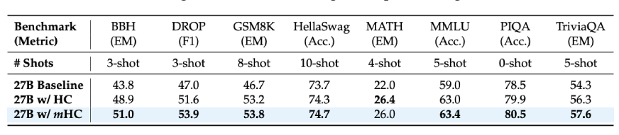


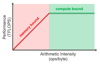

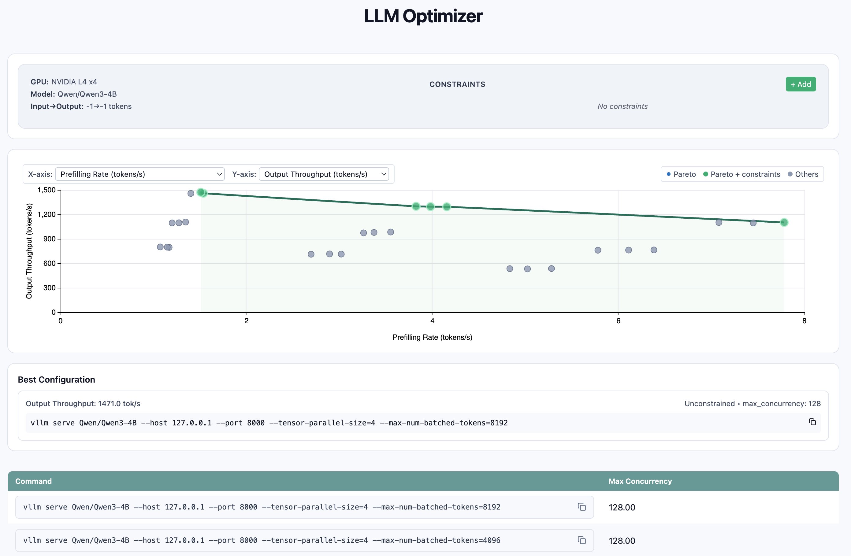
 Josh Longenecker