OpenAI is reportedly testing a brand new characteristic or product codenamed “Sonata,” and it could possibly be associated to music or audio-related experiences on ChatGPT.
As noticed by Tibor on X, there are contemporary OpenAI-related hostnames noticed just lately.
The primary is sonata.openai.com (dated 2026-01-16) and sonata.api.openai.com (dated 2026-01-15).
This implies OpenAI (or its infrastructure) has began utilizing a brand new subdomain, “sonata,” on each its predominant area and its API area.
A brand new hostname means OpenAI is testing a brand new service. OpenAI hostnames usually level to a web-facing product web page, inside software, or an internet app.
The codename is “sonata,” which refers to a multi-movement instrumental music composition. Nevertheless, it can confer with different issues too (like a automobile mannequin, an organization identify, or a drug model).
It is a good reminder {that a} codename doesn’t inform you what the characteristic is.
“When reference chat historical past is enabled, ChatGPT can now extra reliably discover particular particulars out of your previous chats whenever you ask,” OpenAI confirmed in up to date launch notes.
Any previous chat used to reply your query now seems as a supply, so you possibly can open and overview the unique context.
OpenAI can be enhancing dictation capabilities in ChatGPT for all logged-in customers.
As MCP (Mannequin Context Protocol) turns into the usual for connecting LLMs to instruments and information, safety groups are shifting quick to maintain these new companies secure.
This free cheat sheet outlines 7 greatest practices you can begin utilizing in the present day.
There’s no denying the attract of alien artifacts. Science fiction is awash within the materials remnants of extraterrestrial civilizations, which floor in the whole lot from the basic books of Arthur C. Clarke to sport franchises like Mass Impact and Outer Wilds.
The invention of the primary interstellar objects within the photo voltaic system inside the previous decade has sparked hypothesis that they may very well be alien artifacts or spaceships, although the scientific consensus stays that each one three of those guests have pure explanations.
That mentioned, scientists have been anticipating the potential of encountering alien artifacts for the reason that daybreak of the area age.
“Within the historical past of technosignatures, the likelihood that there may very well be artifacts within the photo voltaic system has been round for a very long time,” says Adam Frank, a professor of astrophysics on the College of Rochester.
“We have been serious about this for many years. We’ve been ready for this to occur,” he continues. “However being accountable scientists means holding to the very best requirements of proof and in addition not crying wolf.”
That raises some tantalizing questions: What’s one of the best ways to seek for alien artifacts? And what ought to we do if we really establish one? On condition that these technosignatures may run the gamut from tiny alloy flecks to hulking spaceships—or maybe, some materials that’s unimaginable to Earthlings—it’s tough to know what to anticipate.
To satisfy this problem, researchers are at present engaged on an array of methods to seek for indicators of alien remnants throughout our photo voltaic system—together with in orbit round Earth.
For instance, Beatriz Villarroel, an assistant professor of astronomy on the Nordic Institute for Theoretical Physics, has centered on a largely untapped observational useful resource: historic photos of the sky taken earlier than the human area age.
By finding out archival photographic observations captured by telescopes previous to the launch of Sputnik in 1957, Villarroel has produced a portrait of the sky earlier than it was speckled with our satellites. Because the lead of the Vanishing & Showing Sources throughout a Century of Observations venture (VASCO), she had initially been on the lookout for any proof that stars, or different pure objects, would possibly vanish on these archival plates.
As an alternative Villarroel discovered inexplicable “transients” that appear to be synthetic satellites in orbit round Earth, lengthy earlier than the launch of Sputnik, which she and her colleagues reported in 2021.
“That’s once I realized that is really a implausible archive, not for trying to find vanishing stars, however for on the lookout for artifacts,” she says.
The thriller may probably be resolved with a devoted mission to seek for artifacts in geosynchronous orbit, an setting about 22,000 miles above Earth. Nevertheless, Villarroel doubts that such a mission could be green-lit by any federal area company within the close to time period, as a result of controversial nature of the subject.
“There’s a lot taboo that no one’s ever going to take such outcomes critically till you carry down such a probe,” she provides.
Frank says he agrees that the stigmatization of the seek for otherworldly artifacts—and the seek for alien life, extra broadly—is counterproductive. However he sees the pushback over analysis into alien artifacts as a wholesome and pure a part of scientific inquiry.
When one analyzes a number of time sequence, the pure extension to the autoregressive mannequin is the vector autoregression, or VAR, through which a vector of variables is modeled as relying on their very own lags and on the lags of each different variable within the vector. A two-variable VAR with one lag appears like
Utilized macroeconomists use fashions of this way to each describe macroeconomic knowledge and to carry out causal inference and supply coverage recommendation.
On this publish, I’ll estimate a three-variable VAR utilizing the U.S. unemployment price, the inflation price, and the nominal rate of interest. This VAR is just like these utilized in macroeconomics for financial coverage evaluation. I focus on fundamental points in estimation and postestimation. Information and do-files are offered on the finish. Extra background and theoretical particulars could be present in Ashish Rajbhandari’s [earlier post], which explored VAR estimation utilizing simulated knowledge.
Information and estimation
When writing down a VAR, one makes two fundamental model-selection decisions. First, one chooses which variables to incorporate within the VAR. This determination is usually motivated by the analysis query and guided by idea. Second, one chooses the lag size. Heuristics could also be used, similar to “embody one 12 months value of lags”, or there are formal lag-length choice standards accessible. As soon as the lag size has been decided, one could proceed to estimation; as soon as the parameters of the VAR have been estimated, one can carry out postestimation procedures to evaluate mannequin match.
I exploit quarterly observations on the U.S. unemployment price, price of client value inflation, and short-term nominal rate of interest from 1955 to 2005. The three sequence have been downloaded from the Federal Reserve Financial Database at https://fred.stlouisfed.org. Within the Stata output that follows, the inflation price is known as inflation, the unemployment price as unrate, and the rate of interest as ffr (federal funds price). Therefore, the VAR I’ll estimate is start{align} start{bmatrix} {bf inflation}_t {bf unrate}_t {bf ffr}_t finish{bmatrix} = {bf a_0} + {bf A_1} start{bmatrix} {bf inflation}_{t-1} {bf unrate}_{t-1} {bf ffr}_{t-1} finish{bmatrix} + dots + {bf A_k} start{bmatrix} {bf inflation}_{t-k} {bf unrate}_{t-k} {bf ffr}_{t-k} finish{bmatrix} + start{bmatrix} varepsilon_{1,t} varepsilon_{2,t} varepsilon_{3,t} finish{bmatrix} finish{align} ({bf a_0}) is a vector of intercept phrases and every of ({bf A_1}) to ({bf A_k}) is a (3 occasions 3) matrix of coefficients. VARs with these variables, or shut analogues to them, are widespread in financial coverage evaluation.
The subsequent step is to resolve on a wise lag size. I exploit the varsoc command to run lag-order choice diagnostics.
varsoc shows the outcomes of a battery of lag-order choice exams. The small print of those exams could also be present in assist varsoc. Each the chance ratio take a look at and Akaike’s info criterion suggest six lags, which I exploit by way of the remainder of this publish.
With variables and lag size in hand, there are two objects to estimate: the coefficient matrices and the covariance matrix of the error phrases. Coefficients could be estimated by least squares, equation by equation. The covariance matrix of the errors could also be estimated from the pattern covariance matrix of the residuals. var performs each duties.
The desk of coefficients is displayed by default, and the covariance estimate of the error phrases could be discovered within the saved outcome e(Sigma):
The output of var organizes its outcomes by equation, the place an “equation” is recognized with its dependent variable: therefore, there may be an inflation equation, an unemployment equation, and an rate of interest equation. e(Sigma) holds the covariance matrix of the estimated residuals from the VAR. Notice that the residuals are correlated throughout equations.
As you may anticipate, the desk of coefficients is fairly lengthy. Not together with the fixed phrases, a VAR with (n) variables and (okay) lags could have (kn^2) coefficients; our 3-variable, 6-lag VAR has almost 60 coefficients which are estimated with solely 198 observations. The choices dfk and small apply small-sample corrections to the large-sample statistics which are reported by default. We are able to look down the desk of coefficients, commonplace errors, t statistics, and p-values, however it’s not instantly informative to take a look at the coefficients on particular person covariates in isolation. Due to this, many utilized papers don’t even report the desk of coefficients; as a substitute, they report some postestimation statistics which are (hopefully) extra informative. The subsequent two sections will discover two widespread postestimation statistics which are used to evaluate VAR output: Granger causality exams and impulse–response features.
Evaluating the output of a VAR: Granger causality exams
A variable (x_t) is claimed to “Granger-cause” one other variable (y_t) if, given the lags of (y_t), the lags of (x_t) are collectively statistically vital within the (y_t) equation. For instance, the rate of interest Granger-causes unemployment if lags of the rate of interest are collectively statistically vital within the unemployment equation. The vargranger postestimation command performs a battery of Granger causality exams.
As earlier than, equations are distinguished by their dependent variable. For every equation, vargranger exams for the Granger causality of every variable within the VAR individually, then exams for the Granger causality of all added variables collectively. Take into account the Granger causality exams for the unemployment equation. The row with “ffr excluded” exams the null speculation that each one coefficients on lags of the rate of interest within the unemployment equation are equal to zero, towards the choice that at the least one shouldn’t be equal to zero. The p-value of 0.27 doesn’t fall under the standard statistical significance threshold of 0.05; therefore, we can not reject the null speculation that lags of the rate of interest don’t have an effect on the unemployment price. With this mannequin and these knowledge, the rate of interest doesn’t Granger-cause unemployment. In contrast, within the rate of interest equation, lags of each inflation and unemployment are statistically vital and could be mentioned to Granger-cause the rate of interest.
The “all excluded” row for every equation excludes all lags that aren’t the autocorrelation coefficients in an equation; it’s a joint take a look at for the importance of all lags of all different variables in that equation. It could be thought-about a take a look at between a purely autoregressive specification (null) towards the VAR specification for that equation (alternate).
You’ll be able to replicate the outcomes of the Granger causality exams by operating bizarre least squares on every equation and utilizing take a look at with the suitable null speculation:
The outcomes of a “handbook” Granger causality take a look at match the outcomes from vargranger.
Evaluating the output of a VAR: Impulse responses
The second set of statistics usually used to evaulate a VAR is to simulate some shocks to the system and hint out the results of these shocks on endogenous variables. However do not forget that the shocks have been correlated throughout equations,
and it’s ambiguous to speak a couple of “shock” to, say, the inflation equation when the error phrases are correlated throughout equations.
One method to this drawback is to suppose that there are underlying structural shocks (bf{u}_t), that are (by definition) uncorrelated, and that these shocks are associated to the reduced-form shocks by way of the next relationship:
Many (bf{A}) matrices fulfill (1). One method to slender down the attainable candidates is to imagine that (bf{A}) is lower-triangular; then (bf{A}) could be discovered uniquely by way of a Cholesky decomposition of (bf{Sigma}). This method is so widespread that it’s constructed into the var postestimation outcomes and could be accessed straight.
The belief that (bf{A}) is lower-triangular imposes an ordering on the variables within the VAR, and totally different orderings will produce totally different (bf{A}). The financial content material of this ordering is that the shock to anybody equation impacts the variables later within the ordering contemporaneously however that every variable within the VAR is contemporaneously unaffected by the shocks to the equations above it. For this publish, I’ll impose the ordering we’ve used to date: the equations are ordered inflation first, then unemployment, then the rate of interest. The inflation shock is allowed to have an effect on all three variables contemporaneously; the unemployment shock is allowed to have an effect on the rate of interest contemporaneously, however not inflation; and the rate of interest shock comes “final” and doesn’t have an effect on both inflation or unemployment contemporaneously.
With (bf{A}) in hand, we are able to produce shocks which are uncorrelated throughout equations and hint out the results of these shocks on the variables within the VAR. We are able to construct the impulse–response features with irf create, then graph the output with irf graph.
. quietly var inflation unrate ffr, lags(1/6) dfk small

. irf create var1, step(20) set(myirf) substitute
(file myirf.irf now energetic)
(file myirf.irf up to date)

. irf graph oirf, impulse(inflation unrate ffr) response(inflation unrate ffr)
>         yline(0,lcolor(black)) xlabel(0(4)20) byopts(yrescale)
After operating the VAR, irf create creates an .irf file that shops quite a few outcomes from the VAR that could be of curiosity in postestimation. The outcomes of multiple VAR could also be saved in a single .irf file, so we give the VAR a reputation, on this case var1. The set() possibility names the .irf file—on this case myirf.irf—and units it because the “energetic” .irf file for the needs of later postestimation instructions. The step(20) possibility instructs irf create to generate sure statistics, similar to forecasts, out to a horizon of 20 durations.
The irf graph command graphs among the statistics saved within the .irf file. Of the various statistics in that file, we can be within the orthogonalized impulse–response perform, so we specify oirf, therefore, the command irf graph oirf. The impulse() and response() choices specify which equations to shock and which variables to graph; we are going to shock all equations and graph all variables.
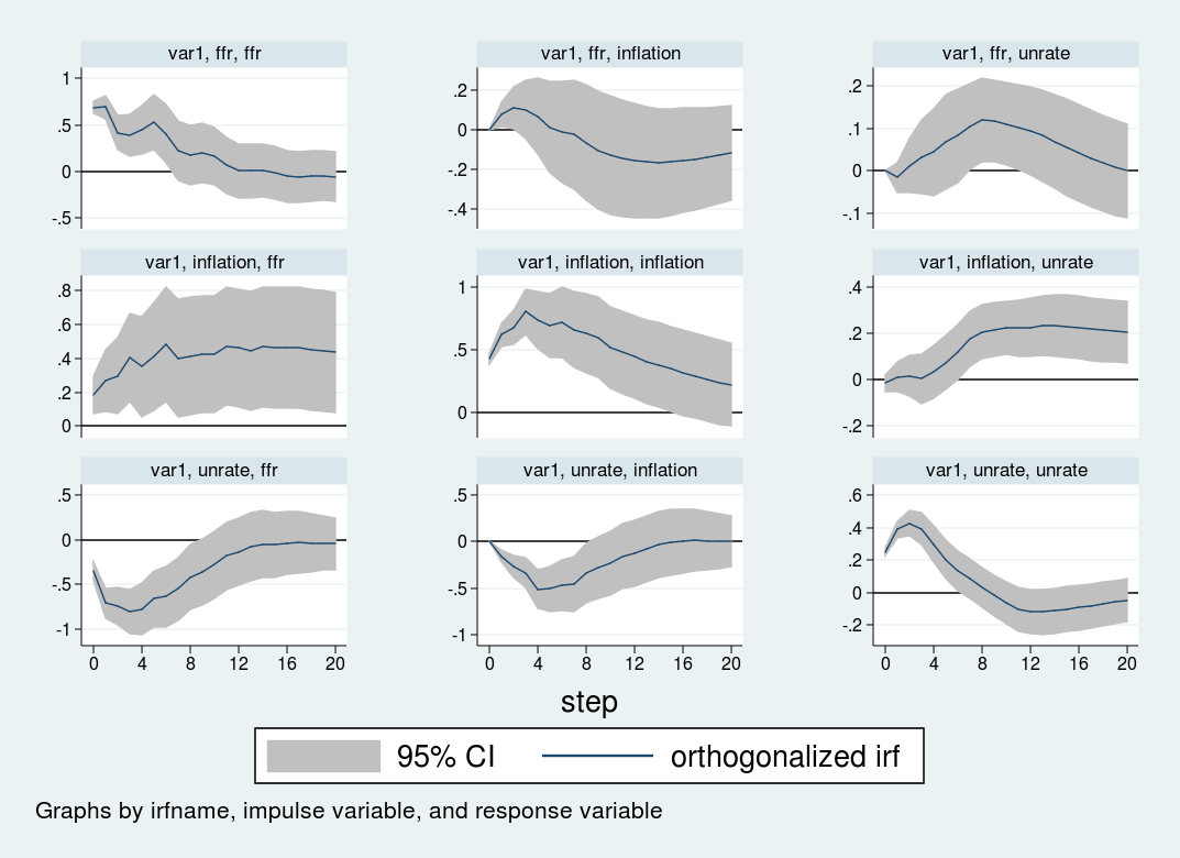
The impulse–response graphs are the next:
The impulse–response graph locations one impulse in every row and one response variable in every column. The horizontal axis for every graph is within the items of time that your VAR is estimated in, on this case quarters; therefore, the impulse–response graph exhibits the impact of a shock over a 20-quarter interval. The vertical axis is in items of the variables within the VAR; on this case, every thing is measured in proportion factors, so the vertical items in all panels are proportion level adjustments.
The primary row exhibits the impact of a one-standard-deviation impulse to the rate of interest equation. The rate of interest is persistent and stays elevated for about 12 durations (3 years) after the preliminary impulse. Inflation declines barely after eight quarters, however the response shouldn’t be statistically vital at any horizon. The unemployment price rises slowly for about 12 durations, peaking at a 0.2 perentage level improve, earlier than declining.
The second row exhibits the impression of a shock to the inflation equation. An sudden improve in inflation is related to a extremely persistent improve within the unemployment price and the rate of interest. Each the rate of interest and unemployment price stay elevated even 5 years after the impulse to inflation.
Lastly, the third row exhibits the impression to a shock to the unemployment equation. An impulse to the unemployment price causes inflation to say no by about one half of 1 proportion level over the next 12 months. The rate of interest responds strongly to the unemployment shock, falling by almost one proportion level over the 12 months following the shock.
Each the VAR and the ordering used listed here are illustrative. All of the inferences are conditional on the (bf{A}) matrix, that’s, the ordering of the variables within the VAR. Totally different orderings will produce totally different (bf{A}) matrices, which in flip will produce totally different impulse responses. As well as, there are identification methods that transcend merely ordering the equations; I’ll talk about these strategies in a later publish.
Conclusion
On this publish, I estimated a VAR mannequin and mentioned two widespread postestimation statistics: Granger causality exams and impulse–response features. In my subsequent publish, I’ll go deeper into the impulse response perform and describe different identification methods for performing structural inference in a VAR.
I first heard about Epicor’s choice when one in every of my long-time purchasers, an organization for whom ERP reliability is mission-critical, reached out with deep issues. Like so many others, they’re being pushed into the cloud not by optimistic enterprise drivers, however by the withdrawal of the on-premises choice. Their worries are removed from theoretical. Simply final 12 months, main outages reminded us that the cloud, for all its strengths, is not any panacea for threat. Add reputable worries about latency, compliance, and new safety fashions, and it’s clear that this transition creates nervousness proper alongside alternative.
Let’s be clear about what’s motivating this pattern. For Epicor and its friends, shifting to SaaS means they will focus their assets, decrease help prices, speed up innovation, and simplify patching, safety, and integrations. With Epicor Cloud, for instance, each buyer runs the identical core code, patches are pushed universally, and working bills fall consequently. It’s a sound enterprise technique for distributors to achieve recurring income, much less model sprawl, and a extra streamlined engineering group.
That effectivity usually comes on the expense of buyer alternative. Enterprises are requested to cede infrastructure management, settle for new dependencies, and belief that the vendor-managed setting will meet all their necessities for safety, latency, uptime, and regulatory compliance—typically with solely restricted visibility or contractual recourse. For organizations that chosen on-prem software program exactly due to their distinctive wants, it is a seismic change that may’t be solved by merely “lifting and shifting” their functions.
Most Python builders deal with logging as an afterthought. They throw round print() statements throughout improvement, possibly change to fundamental logging later, and assume that’s sufficient. However when points come up in manufacturing, they be taught they’re lacking the context wanted to diagnose issues effectively.
Correct logging strategies provide you with visibility into software conduct, efficiency patterns, and error situations. With the suitable method, you’ll be able to hint consumer actions, determine bottlenecks, and debug points with out reproducing them domestically. Good logging turns debugging from guesswork into systematic problem-solving.
This text covers the important logging patterns that Python builders can use. You’ll learn to construction log messages for searchability, deal with exceptions with out shedding context, and configure logging for various environments. We’ll begin with the fundamentals and work our manner as much as extra superior logging methods that you need to use in initiatives instantly. We shall be utilizing solely the logging module.
As a substitute of leaping straight to complicated configurations, allow us to perceive what a logger truly does. We’ll create a fundamental logger that writes to each the console and a file.
import logging

logger = logging.getLogger('my_app')
logger.setLevel(logging.DEBUG)

console_handler = logging.StreamHandler()
console_handler.setLevel(logging.INFO)

file_handler = logging.FileHandler('app.log')
file_handler.setLevel(logging.DEBUG)

formatter = logging.Formatter(
    '%(asctime)s - %(identify)s - %(levelname)s - %(message)s'
)
console_handler.setFormatter(formatter)
file_handler.setFormatter(formatter)

logger.addHandler(console_handler)
logger.addHandler(file_handler)

logger.debug('It is a debug message')
logger.data('Utility began')
logger.warning('Disk house operating low')
logger.error('Failed to connect with database')
logger.essential('System shutting down')
Here’s what each bit of the code does.
The getLogger() operate creates a named logger occasion. Consider it as making a channel in your logs. The identify ‘my_app’ helps you determine the place logs come from in bigger functions.
We set the logger stage to DEBUG, which suggests it can course of all messages. Then we create two handlers: one for console output and one for file output. Handlers management the place logs go.
The console handler solely exhibits INFO stage and above, whereas the file handler captures every part, together with DEBUG messages. That is helpful since you need detailed logs in information however cleaner output on display.
The formatter determines how your log messages look. The format string makes use of placeholders like %(asctime)s for the timestamp and %(levelname)s for severity.
# Understanding Log Ranges and When to Use Every
Python’s logging module has 5 normal ranges, and understanding when to make use of each is necessary for helpful logs.
Allow us to break down when to make use of every stage:
DEBUG is for detailed info helpful throughout improvement. You’d use it for variable values, loop iterations, or step-by-step execution traces. These are often disabled in manufacturing.
INFO marks regular operations that you simply wish to report. Beginning a server, finishing a activity, or profitable transactions go right here. These verify your software is working as anticipated.
WARNING indicators one thing sudden however not breaking. This contains low disk house, deprecated API utilization, or uncommon however dealt with conditions. The applying continues operating, however somebody ought to examine.
ERROR means one thing failed however the software can proceed. Failed database queries, validation errors, or community timeouts belong right here. The particular operation failed, however the app retains operating.
CRITICAL signifies critical issues which may trigger the applying to crash or lose knowledge. Use this sparingly for catastrophic failures that want quick consideration.
If you run the above code, you’ll get:
DEBUG: Beginning fee processing for consumer 12345
DEBUG:payment_processor:Beginning fee processing for consumer 12345
INFO: Processing $150.0 fee for consumer 12345
INFO:payment_processor:Processing $150.0 fee for consumer 12345
INFO: Fee profitable for consumer 12345
INFO:payment_processor:Fee profitable for consumer 12345
DEBUG: Beginning fee processing for consumer 12345
DEBUG:payment_processor:Beginning fee processing for consumer 12345
INFO: Processing $15000.0 fee for consumer 12345
INFO:payment_processor:Processing $15000.0 fee for consumer 12345
WARNING: Giant transaction detected: $15000.0
WARNING:payment_processor:Giant transaction detected: $15000.0
INFO: Fee profitable for consumer 12345
INFO:payment_processor:Fee profitable for consumer 12345
True
Subsequent, allow us to proceed to know extra about logging exceptions.
# Logging Exceptions Correctly
When exceptions happen, you want extra than simply the error message; you want the total stack hint. Right here is the best way to seize exceptions successfully.
The important thing right here is the exc_info=True parameter. This tells the logger to incorporate the total exception traceback in your logs. With out it, you solely get the error message, which regularly shouldn’t be sufficient to debug the issue.
Discover how we catch particular exceptions first, then have a basic Exception handler. The particular handlers allow us to present context-appropriate error messages. The final handler catches something sudden and re-raises it as a result of we have no idea the best way to deal with it safely.
Additionally discover we log at ERROR for anticipated exceptions (like community errors) however CRITICAL for sudden ones. This distinction helps you prioritize when reviewing logs.
# Making a Reusable Logger Configuration
Copying logger setup code throughout information is tedious and error-prone. Allow us to create a configuration operate you’ll be able to import wherever in your undertaking.
# logger_config.py

import logging
import os
from datetime import datetime


def setup_logger(identify, log_dir="logs", stage=logging.INFO):
    """
    Create a configured logger occasion

    Args:
        identify: Logger identify (often __name__ from calling module)
        log_dir: Listing to retailer log information
        stage: Minimal logging stage

    Returns:
        Configured logger occasion
    """
    # Create logs listing if it would not exist

    if not os.path.exists(log_dir):
        os.makedirs(log_dir)
    logger = logging.getLogger(identify)

    # Keep away from including handlers a number of instances

    if logger.handlers:
        return logger
    logger.setLevel(stage)

    # Console handler - INFO and above

    console_handler = logging.StreamHandler()
    console_handler.setLevel(logging.INFO)
    console_format = logging.Formatter("%(levelname)s - %(identify)s - %(message)s")
    console_handler.setFormatter(console_format)

    # File handler - every part

    log_filename = os.path.be a part of(
        log_dir, f"{identify.exchange('.', '_')}_{datetime.now().strftime('%Ypercentmpercentd')}.log"
    )
    file_handler = logging.FileHandler(log_filename)
    file_handler.setLevel(logging.DEBUG)
    file_format = logging.Formatter(
        "%(asctime)s - %(identify)s - %(levelname)s - %(funcName)s:%(lineno)d - %(message)s"
    )
    file_handler.setFormatter(file_format)

    logger.addHandler(console_handler)
    logger.addHandler(file_handler)

    return logger
Now that you’ve arrange logger_config, you need to use it in your Python script like so:
This setup operate handles a number of necessary issues. First, it creates the logs listing if wanted, stopping crashes from lacking directories.
The operate checks if handlers exist already earlier than including new ones. With out this verify, calling setup_logger a number of instances would create duplicate log entries.
We generate dated log filenames robotically. This prevents log information from rising infinitely and makes it straightforward to seek out logs from particular dates.
The file handler contains extra element than the console handler, together with operate names and line numbers. That is invaluable when debugging however would litter console output.
Utilizing __name__ because the logger identify creates a hierarchy that matches your module construction. This allows you to management logging for particular elements of your software independently.
# Structuring Logs with Context
Plain textual content logs are high-quality for easy functions, however structured logs with context make debugging a lot simpler. Allow us to add contextual info to our logs.
import json
from datetime import datetime, timezone

class ContextLogger:
    """Logger wrapper that provides contextual info to all log messages"""

    def __init__(self, identify, context=None):
        self.logger = logging.getLogger(identify)
        self.context = context or {}

        handler = logging.StreamHandler()
        formatter = logging.Formatter('%(message)s')
        handler.setFormatter(formatter)
        # Test if handler already exists to keep away from duplicate handlers
        if not any(isinstance(h, logging.StreamHandler) and h.formatter._fmt == '%(message)s' for h in self.logger.handlers):
            self.logger.addHandler(handler)
        self.logger.setLevel(logging.DEBUG)

    def _format_message(self, message, stage, extra_context=None):
        """Format message with context as JSON"""
        log_data = {
            'timestamp': datetime.now(timezone.utc).isoformat(),
            'stage': stage,
            'message': message,
            'context': {**self.context, **(extra_context or {})}
        }
        return json.dumps(log_data)

    def debug(self, message, **kwargs):
        self.logger.debug(self._format_message(message, 'DEBUG', kwargs))

    def data(self, message, **kwargs):
        self.logger.data(self._format_message(message, 'INFO', kwargs))

    def warning(self, message, **kwargs):
        self.logger.warning(self._format_message(message, 'WARNING', kwargs))

    def error(self, message, **kwargs):
        self.logger.error(self._format_message(message, 'ERROR', kwargs))
This ContextLogger wrapper does one thing helpful: it robotically contains context in each log message. The order_id and user_id get added to all logs with out repeating them in each logging name.
The JSON format makes these logs straightforward to parse and search.
The **kwargs in every logging technique enables you to add further context to particular log messages. This combines international context (order_id, user_id) with native context (item_count, whole) robotically.
This sample is very helpful in internet functions the place you need request IDs, consumer IDs, or session IDs in each log message from a request.
# Rotating Log Information to Forestall Disk Area Points
Log information develop rapidly in manufacturing. With out rotation, they may ultimately fill your disk. Right here is the best way to implement automated log rotation.
Allow us to now attempt to use rotation of log information:
for i in vary(1000):
    logger.data(f'Processing report {i}')
    logger.debug(f'File {i} particulars: accomplished in {i * 0.1}ms')
RotatingFileHandler manages logs based mostly on file dimension. When the log file reaches 10MB (laid out in bytes), it will get renamed to app_size_rotation.log.1, and a brand new app_size_rotation.log begins. The backupCount of 5 means you’ll hold 5 outdated log information earlier than the oldest will get deleted.
TimedRotatingFileHandler rotates based mostly on time intervals. The ‘midnight’ parameter means it creates a brand new log file each day at midnight. You would additionally use ‘H’ for hourly, ‘D’ for day by day (at any time), or ‘W0’ for weekly on Monday.
The interval parameter works with the when parameter. With when='H' and interval=6, logs would rotate each 6 hours.
These handlers are important for manufacturing environments. With out them, your software might crash when the disk fills up with logs.
# Logging in Completely different Environments
Your logging wants differ between improvement, staging, and manufacturing. Right here is the best way to configure logging that adapts to every surroundings.
This environment-based configuration handles every stage otherwise. Improvement exhibits every part on the console with detailed info, together with operate names and line numbers. This makes debugging quick.
Staging balances improvement and manufacturing. It writes detailed logs to information for investigation however solely exhibits warnings and errors on the console to keep away from noise.
Manufacturing focuses on efficiency and construction. It solely logs INFO stage and above to information, makes use of JSON formatting for straightforward parsing, and implements log rotation to handle disk house. Console output is restricted to errors solely.
# Set surroundings variable (usually achieved by deployment system)
os.environ['APP_ENV'] = 'manufacturing'

logger = configure_environment_logger('my_application')

logger.debug('This debug message will not seem in manufacturing')
logger.data('Consumer logged in efficiently')
logger.error('Didn't course of fee')
The surroundings is decided by the APP_ENV surroundings variable. Your deployment system (Docker, Kubernetes, or different cloud platforms) units this variable robotically.
Discover how we clear current handlers earlier than configuration. This prevents duplicate handlers if the operate is named a number of instances throughout the software lifecycle.
# Wrapping Up
Good logging makes the distinction between rapidly diagnosing points and spending hours guessing what went flawed. Begin with fundamental logging utilizing acceptable severity ranges, add structured context to make logs searchable, and configure rotation to forestall disk house issues.
The patterns proven right here work for functions of any dimension. Begin easy with fundamental logging, then add structured logging while you want higher searchability, and implement environment-specific configuration while you deploy to manufacturing.
Completely satisfied logging!
Bala Priya C is a developer and technical author from India. She likes working on the intersection of math, programming, knowledge science, and content material creation. Her areas of curiosity and experience embrace DevOps, knowledge science, and pure language processing. She enjoys studying, writing, coding, and low! Presently, she’s engaged on studying and sharing her data with the developer neighborhood by authoring tutorials, how-to guides, opinion items, and extra. Bala additionally creates partaking useful resource overviews and coding tutorials.
Paying for Adobe Acrobat month after month can really feel unavoidable—till you keep in mind it’s simply a PDF software program! In case you’re able to cease renting fundamental doc instruments, a PDF Professional lifetime subscription is an easier various that covers the necessities with a one-time buy.
A PDF editor that lasts for all times
PDF Professional handles modifying, signing, changing, and organizing PDFs with out the litter or recurring charges. You’ll be able to repair typos, insert pictures, rearrange pages, merge paperwork, and convert information into Phrase, Excel, or PowerPoint with only a few clicks. It additionally helps type filling and digital signatures.
The OCR characteristic makes scanned PDFs truly usable by turning pictures into searchable, selectable textual content, so you’ll be able to copy content material or discover what you want with out trouble. The interface is quick, clear, and feels prefer it was constructed for macOS, not simply tailored from one thing else.
This model of PDF Professional is a lifetime plan for brand spanking new customers, that means you pay as soon as and use it for so long as you want. You’ll get common updates and help, however you gained’t be locked into one other auto-renewing subscription.
An earthquake-generating chunk of tectonic plate has been found beneath Northern California. It’s hooked up to the underside of the North American plate like gum caught to a shoe.
Utilizing plentiful, tiny, almost imperceptible earthquakes that may assist reveal sophisticated faults beneath Earth’s floor, researchers have recognized this beforehand hidden hazard. The plate might have been the supply of the 1992 magnitude 7.2 Mendocino earthquake, researchers report January 15 in Science.
Beneath the peaceable great thing about Northern California’s Misplaced Coast lies a sophisticated, stressed geologic jumble, one of many United States’ most lively tectonic areas. It’s the place the San Andreas Fault meets the Cascadia subduction zone. Three sections of Earth’s crust meet on this area, a conflict of titans generally known as the Mendocino triple junction: the North American Plate and the Pacific Plate are sideswiping one another, whereas the smaller Gorda Plate is diving beneath the North American slab.
In 1992, a magnitude 7.2 earthquake rocked the Cape Mendocino area, damaging buildings and roads and triggering landslides and a small tsunami. Surprisingly for such a big quake, the epicenter turned out to be solely about 10 kilometers deep, puzzling scientists; the subducting slab of the Gorda plate was recognized to be at the least twice as deep.
Some proposed {that a} “slab hole” existed, a shallow house shaped by the friction of 1 plate dragging one other, with mantle magma welling up into that window and producing quakes. However one other chance was that there was one thing else down there: a fraction of tectonic plate.
Tectonic site visitors jam
The Mendocino triple junction is a sophisticated jumble of colliding plates of Earth’s crust. Black arrows depict actions relative to the North American Plate: The Pacific Plate is sideswiping it, creating the San Andreas Fault system, whereas the Gorda Plate is sinking beneath it on the Cascadia subduction zone. Blue arrows point out how the Pacific and Gorda plates are transferring sideways previous one another. Utilizing tiny earthquakes generated close to the southern fringe of the Gorda Plate (in pink), researchers found the “Pioneer” fragment, a remnant of the traditional Farallon Plate that’s getting dragged beneath the North American Plate.
David Shelly/USGSDavid Shelly/USGS
The dwindling Gorda Plate is definitely one of many final remnants of the traditional Farallon Plate. Most of it has descended into the mantle — however a fraction of it may need gotten trapped throughout subduction and pasted on to the overlying North American plate because it grinded by. And now that fragment could also be getting dragged alongside on the underside of the plate
Easy methods to see that hidden fragment was the issue — it’s probably not seen from the floor, say U.S. Geological Survey geophysicist David Shelly, based mostly in Golden, Colo., and colleagues. The staff determined to visualize the area’s complicated tectonics utilizing swarms of tiny earthquakes. These quakes are imperceptible to people however detectable by seismometers; they recur quickly, forming a long-duration seismic sign generally known as a tremor. By “stacking” the plentiful occurrences of those occasions, researchers can decide a extra exact depth and site for each, finally delineating fault strains and different subsurface options.
The staff zoomed in on a area of tremor close to the southern fringe of the subducting Gorda Plate. The tiny earthquakes, they discovered, have been generated by a sideways-moving little bit of crust, situated about 10 kilometers under the floor. That, the staff suggests, factors to a separate plate fragment shallower than the subducting slab. They dubbed it the Pioneer fragment.
By figuring out this hidden fragment, the staff has additionally basically found a buried plate boundary, an almost horizontal fault line between the Pioneer fragment and the overlying North American plate that may be a supply of robust however shallow earthquakes — just like the 1992 Cape Mendocino quake.
That might imply the triple junction is extra of a quadruple junction — however in reality there’s a fifth stray little bit of tectonic plate hidden below the floor, the researchers say. Beneath the southern finish of the Cascadia subduction zone is one other buried fragment of crust, a piece of the North American Plate that broke off the primary plate and is now getting tugged down into the mantle by the sinking Gorda Plate.
Shining a light-weight into the subsurface of this area helps determine and put together for beforehand unknown seismic hazards, says Matthew Herman, a geophysicist at California State College, Bakersfield who was not a part of the brand new examine.
“We frequently view triple junction areas as a easy intersection of three easy plate boundary types,” Herman says. This examine “is a part of a rising physique of analysis displaying we can not perceive the entire image” with out understanding how Cascadia subduction interacts with the San Andreas Fault system. “This Pioneer fragment … might pose a distinctly totally different kind of earthquake hazard than we anticipate.”
Recurrent Neural Networks (RNNs) laid the muse for sequence modeling, however their intrinsic sequential nature restricts parallel computation, making a basic barrier to scaling. This has led to the dominance of parallelizable architectures like Transformers and, extra lately, State House Fashions (SSMs). Whereas SSMs obtain environment friendly parallelization by structured linear recurrences, this linearity constraint limits their expressive energy and precludes modeling advanced, nonlinear sequence-wise dependencies. To handle this, we current ParaRNN, a framework that breaks the sequence-parallelization barrier for nonlinear RNNs. Constructing on prior work, we solid the sequence of nonlinear recurrence relationships as a single system of equations, which we remedy in parallel utilizing Newton’s iterations mixed with customized parallel reductions. Our implementation achieves speedups of as much as 665x over naive sequential software, permitting coaching nonlinear RNNs at unprecedented scales. To showcase this, we apply ParaRNN to diversifications of LSTM and GRU architectures, efficiently coaching fashions of 7B parameters that attain perplexity similar to similarly-sized Transformers and Mamba2 architectures. To speed up analysis in environment friendly sequence modeling, we launch the ParaRNN codebase as an open-source framework for automated training-parallelization of nonlinear RNNs, enabling researchers and practitioners to discover new nonlinear RNN fashions at scale.
I’ve combed the web to search out you in the present day’s most enjoyable/vital/scary/fascinating tales about know-how.
1 Iran is systematically crippling Starlink The satellite tv for pc web service is supposed to be inconceivable to jam—however the Iranian authorities are doing simply that. (Remainder of World) + Messages getting round Iran’s web block recommend that 1000’s of individuals have been killed. (NYT $) + On the bottom in Ukraine’s largest Starlink restore store. (MIT Expertise Assessment)
2 Research claiming microplastics hurt us are being referred to as into query Some scientists say the discoveries are most likely the results of contamination and false positives. (The Guardian)
3 Trump is attempting to mood the info heart backlash He hopes cajoling tech firms to pay extra and thus cut back folks’s power payments will do the trick. (WP $) + Microsoft has simply change into the primary tech firm to vow it’ll do exactly that. (NYT $) + We all know AI is energy hungry. However simply how massive is the size of the issue? (MIT Expertise Assessment)
4 US emissions jumped final yr Because of a mix of rising electrical energy demand, and extra coal being burned to satisfy it. (NYT $) + However it’s not all unhealthy information: coal energy era in India and China lastly began to say no. (The Guardian) + 4 shiny spots in local weather information in 2025. (MIT Expertise Assessment)
5 Elon Musk must face penalties for his actions If we tolerate him unleashing a flood of harassment of ladies and kids, what is going to come subsequent? (The Atlantic $) + The US Senate has handed a invoice that would give non-consensual deepfake victims a brand new approach to struggle again. (The Verge $)
6 Why the US is ready to lose the race again to the moon 🚀🌔 Cuts to NASA aren’t serving to, however they’re not the one drawback. (Wired $)
7 Google’s Veo AI mannequin can now flip portrait photographs into vertical movies Actually slick ones, too. (The Verge $) + AI-generated influencers are sharing pretend photographs of them in mattress with celebrities on Instagram. (404 Media $)
8 Former NYC mayor Eric Adams has been accused of a crypto ‘pump and dump’ He promoted a token that noticed its market cap briefly soar to $580 million earlier than plummeting. (Coindesk)
9 Are you a center supervisor? Right here’s some excellent news for you Your expertise aren’t being changed by AI any time quickly. (Quartz)
10 Even miniscule way of life tweaks can prolong your lifespan A examine of 60,000 adults discovered just a bit bit extra sleep and train makes an enormous distinction. (New Scientist $) + Growing old hits us in our 40s and 60s. However well-being doesn’t should fall off a cliff. (MIT Expertise Assessment)
Our skilled reviewers spend hours testing and evaluating services and products so you possibly can select the most effective for you. Discover out extra about how we check.
The COROS NOMAD is not actually for “nomads.” A real backpacker spending weeks per 12 months within the mountains wants a satellite tv for pc watch (or handheld) for climate alerts, messaging, and SOSs. The NOMAD’s actual target market? Path runners or weekend hikers: individuals keen about health and nature, however who’ll by no means stray too far off the overwhelmed path.
Most adventure-branded watches — the Garmin Fenix 8, Polar Grit X2, Suunto Vertical, or VERTIX 2S — goal severe outdoorsfolk with premium function units and hulking designs. Solely the Garmin Intuition collection caters to the thrifty, average hiker area of interest, and the Intuition 3 strays into mid-range territory.
COROS’s typical enterprise technique is to undercut Garmin’s costs with related options and designs, and the NOMAD performs into that repute. However having used it sporadically over the previous few months, I am genuinely impressed by its worth and efficiency, and it stands out greater than the APEX 4 and PACE 4, COROS’s different 2025 fashions.
COROS NOMAD: Worth and specs
(Picture credit score: COROS)
The COROS NOMAD was launched in mid-August 2025 for $349 / €369 / £319 / CA$499 / AU$649. It is accessible in three finishes: Inexperienced, Brown, and Darkish Gray.
It makes use of the Ambiq Apollo 510 processor, with a Cortex-M55 processor clocked at 250 MHz; for context, the Pixel Watch 4 makes use of the M55 for background duties. A severe velocity improve over previous COROS watches, this processor ensures the NOMAD can have the capability for brand spanking new function upgrades over the subsequent few years.
The NOMAD sports activities the identical sensors, GPS customary, maps, cupboard space, and coaching software program as COROS’s pricier fashions. Upgrading to an APEX 4 or VERTIX 2S primarily nets you titanium supplies, sapphire glass, and longer battery life.
(Picture credit score: Michael Hicks / Android Central)
The NOMAD’s MIP show checks off the proper bins for hikers. COROS tremendously improved the colour and distinction ratio in comparison with older fashions, making it totally readable indoors whereas wanting unbelievable outdoor. It truly beats the pricier APEX 4 for visibility; the latter’s sapphire glass layer provides a reflective tint that dims the distinction.
Get the most recent information from Android Central, your trusted companion on this planet of Android
I will admit to preferring AMOLED shows usually; anybody with poorer eyesight would possibly profit from an Intuition 3 AMOLED, which hits the same three-week lifespan to the NOMAD. However MIP shows are always-on by default, whereas AOD wrecks the Intuition’s battery life. And the latter seems to be a lot dimmer in direct daylight, because it solely hits 1,000 nits. For fast glances whereas operating on tough trails, I would belief the NOMAD extra.
The COROS NOMAD and APEX 4 (Picture credit score: Michael Hicks / Android Central)
COROS lacks the Intuition’s photo voltaic recharging choice, however once more, I do not suppose the goal NOMAD demographic must surpass its spectacular 34-hour dual-band GPS capability — although it could be nearer to 25–30 hours for real-world utilization, primarily based on my testing. Its thick design is not suited to sleep monitoring, so I at all times discover ample time to recharge it within the uncommon moments that it runs low on energy.
Picture 1 of 3
(Picture credit score: Michael Hicks / Android Central)
(Picture credit score: Michael Hicks / Android Central)
(Picture credit score: Michael Hicks / Android Central)
COROS watches won’t ever win magnificence contests, however the polymer-heavy look fits a mountain climbing watch, particularly because the raised bezel protects the show from scratches. I additionally love how the COROS brand is etched subtly into the case, whereas it seems to be cheesy printed in white alongside different fashions’ shows.
At 61g with the silicone band, it is a cheap weight contemplating its dimension, and you should buy an additional nylon band if you wish to slice off 12g. The strap is snug sufficient, although the tip fastening pin takes some getting used to.
(Picture credit score: Michael Hicks / Android Central)
The quick Ambiq processor ensures that turning the crown, or swiping the touchscreen, rapidly scrolls by means of your coaching widgets, well being stats, and primary apps like Calendar and Climate. The UI is straightforward, however streamlined.
COROS added a 3rd Motion button for shortcuts like Laps or Voice Pins throughout actions. It is at present underutilized, however promising: I need the Motion button to assist a number of shortcuts (aka faucet, double-tap, and maintain) and to summon apps exterior of exercises, such because the Compass, Map, or Stopwatch.
(Picture credit score: Michael Hicks / Android Central)
The true NOMAD showstopper is its offline map navigation paired with avenue/path names and close by POIs like bogs or campsites. Obtain your native area, and you may examine which path to tackle impromptu hikes, with near-immediate map loading while you zoom in/out or swipe to pan.
Making a route within the COROS app is straightforward, auto-following trails to particular waypoints, and it syncs to the NOMAD in seconds. With that, you could have clear turn-by-turn navigation to your hike — with warnings if you happen to go off path.
Assuming you pay twice as a lot for a Garmin watch with maps, you will get perks like NextFork warnings at trailheads, ClimbPro knowledge on upcoming hills, or textual content lists of close by or up-ahead POIs that you could navigate on to. However the bloated expertise overloads Garmin’s processor, so it is laggy and irritating to make use of exterior of programs. COROS’s map is less complicated, however works properly, and we are able to hope for map upgrades over time.
Picture 1 of 2
(Picture credit score: Michael Hicks / Android Central)
(Picture credit score: Michael Hicks / Android Central)
Maps apart, the COROS OS focuses on conventional cardio monitoring. The EvoLab coaching suite helps 7-day coaching load with HR zone splits, Coaching Standing, cardio and anaerobic Coaching Impact, restoration estimates, VO2 Max, and different very important stats for severe athletes. Sleep stats like HRV will assist COROS choose your restoration, although once more, not everybody shall be snug sleeping with the NOMAD.
Since August 2025, the NOMAD has added a flashlight show mode, music playback controls, voice coaching notes, transfer alerts, a “Resume Later” software, operating type evaluation, and several other different instruments. I count on the NOMAD’s software program to proceed to enhance over time, catching up in areas the place it falls wanting different manufacturers like Garmin.
COROS NOMAD: GPS accuracy
(Picture credit score: Michael Hicks / Android Central)
My NOMAD health check again in August confirmed how its dual-band GPS and HR accuracy in contrast in opposition to my Garmin Forerunner 970‘s dual-band GPS.
First, throughout a 12-mile run, I used the battery-saving All-Methods mode (with out the L5 GPS frequency), matched in opposition to Garmin’s SatIQ mode for accuracy. They solely differed by 50m/ 0.03 miles, a tiny discrepancy for a protracted distance; the NOMAD (crimson line) often drifted off the highway whereas Garmin’s (blue) stayed regular, but it surely did not affect the general outcomes an excessive amount of.
Picture 1 of 7
(Picture credit score: Android Central)
(Picture credit score: Android Central)
(Picture credit score: Android Central)
(Picture credit score: Android Central)
(Picture credit score: Android Central)
(Picture credit score: Android Central)
(Picture credit score: Android Central)
I toggled dual-band GPS on for each watches on a brief hike loop. Within the more difficult situations, each watches matched my expectations, staying in lockstep with the path. My solely qualm was that the NOMAD’s path (orange) confirmed an odd glitch at hike’s finish, warping me to an earlier a part of the hike (first slide). I have never replicated the error on subsequent hikes, fortunately.
Picture 1 of 5
(Picture credit score: Android Central)
(Picture credit score: Android Central)
(Picture credit score: Android Central)
(Picture credit score: Android Central)
(Picture credit score: Android Central)
I used the NOMAD for 2 different actions, a 10K jog and a seven-mile hike, each utilizing its dual-frequency mode. For the run, each it and the Forerunner 970 measured the identical 6.21 miles and 159 spm cadence, and the NOMAD’s GPS line largely caught to (or near) my real-world path, solely dropping my path in tunnels or beneath some underpasses.
Picture 1 of 2
(Picture credit score: Android Central)
(Picture credit score: Android Central)
For the hike, the NOMAD likewise did properly. It averted any elevation discrepancies that you simply get with much less correct GPS watches and dealt with any sign points beneath foliage or by steep hill faces.
COROS NOMAD: Coronary heart charge accuracy
(Picture credit score: Michael Hicks / Android Central)
Throughout the identical actions above, I synced my Garmin HRM 200 as a management group in opposition to the COROS NOMAD. I by no means count on an optical, wrist-based sensor to match a chest strap completely, however the nearer the typical and smaller the graphical gaps, the higher.
Picture 1 of 2
(Picture credit score: Android Central)
(Picture credit score: Android Central)
Through the 12-mile run (first slide), the NOMAD stayed in parallel with the chest strap, whilst my HR rose from low to excessive cardio and anaerobic; it ended 1 bpm brief on common, however I used to be fairly pleased with the end result.
For the 4-mile hike (second slide), the hole between them was barely extra notable, significantly on sudden inclines or declines, with a couple of HR crests the place the NOMAD did not sustain. It ended 2 bpm brief on common, so I knew I wanted to double-check these outcomes on one other, longer hike.
(Picture credit score: Android Central)
For my subsequent two exams, the NOMAD averaged 1 bpm beneath the Garmin chest strap for my 6-mile run (144 vs. 145), however produced the identical 119-bpm common for my 7-mile hike. Because the above graph exhibits, the NOMAD has a number of moments throughout two hours the place it may possibly’t sustain with the chest strap for sudden rises, but it surely in the end did not have an effect on the final outcomes.
COROS NOMAD: Journey Journal
Picture 1 of 3
(Picture credit score: Michael Hicks / Android Central)
(Picture credit score: Michael Hicks / Android Central)
(Picture credit score: Michael Hicks / Android Central)
COROS gave the NOMAD two signature options: Journey Journal with Voice Pins for hikers and distinctive fishing instruments. I can not communicate to the latter, however the Journey Journal is tailor-made to social media-savvy path runners eager to flaunt their nature exploits, but in addition to on a regular basis hikers.
It is easy sufficient to make use of: Throughout a hike, faucet the NOMAD’s Motion button to both place a pin describing the spot — hazard, toilet, trailfork, and so on. — or file a voice pin as an on-the-go mountain climbing diary entry. When you finish the exercise, COROS can have each pin geotagged in your route, together with your recordings transcribed into textual content.
Voice pins on my route (Picture credit score: Michael Hicks / Android Central)
When you take images or movies, you possibly can assign them to particular pins throughout or after the hike. Then, as soon as your Journal is completed, you simply faucet the Share button, and you may export an information abstract or 3D flyover to publish on-line or share with others.
Some hikers will not care in regards to the sharing side, however it’s useful that pins stay saved in your map; while you construct future routes, you possibly can faucet them to recollect the place you noticed stunning views, tick infestations, or something in-between.
COROS NOMAD: What you will not like
COROS’s UI may use a revamp (Picture credit score: Michael Hicks / Android Central)
Many COROS NOMAD flaws stem from its value: Severe hikers will need sapphire glass or built-in satellite tv for pc connectivity, however these are tall asks for a $350 watch! Nonetheless, potential Garmin converts will miss the built-in flashlight, contactless funds, official MIL-STD-810H ranking, and apps like Spotify and YouTube Music.
My complaints are extra about software program than {hardware}. COROS made this for hikers, however most of its coaching software program stays tailor-made to highway operating greater than path operating, mountain climbing, or rucking. VO2 Max is not tracked for path runs, you possibly can’t add pack weight to regulate your estimates, and restoration estimates take cardiovascular tiredness into consideration greater than muscle fatigue or altitude adjustment. Mainly, the NOMAD may cater to hikers extra than it does now.
Anybody used to an Apple or Put on OS watch will discover COROS’s UI painfully rudimentary. I do not thoughts a streamlined health expertise, however I do discover utilizing the toolbox annoying, in addition to the notification submenu. I would desire an choice to swipe left and proper by means of a couple of favourite apps, or extra app button shortcuts if that is not potential.
The Garmin Intuition 3 is the COROS NOMAD’s essential rival, with kindred designs, the identical core of coaching instruments and exercise plans, and related battery capability and GPS accuracy. Garmin’s mannequin is available in a number of sizes and contains an AMOLED choice, handed the MIL-STD-810H customary check, contains an LED flashlight, and has sure software program perks like every day prompt exercises and a rucking exercise that you will respect. Nevertheless it solely presents breadcrumb navigation, with no offline maps to make complicated trailheads simpler to navigate, and it prices $400–500.
Most different competing journey watches are too costly to be known as “competitors.” An Amazfit T-Rex 3 Professional provides you a rugged design with sapphire glass, as much as 25 days of battery life regardless of the three,000-nit AMOLED show, and features a flashlight, maps, dual-band GPS, and different perks for $400.
COROS NOMAD: Must you purchase it?
(Picture credit score: Michael Hicks / Android Central)
You can purchase the COROS NOMAD if…
You care extra about maps, coaching recs, battery life, and correct outcomes than conventional smarts.
You are prepared to compromise for a lower cost.
You like an MIP show to AMOLED.
You should not purchase the COROS NOMAD if…
You care tremendously about sensible and apps exterior of hikes and exercises.
You are not prepared to surrender a lacking function like sapphire glass, a built-in flashlight, or NFC.
The NOMAD is a superb instance of COROS’s potential to supply nice worth at value tiers that different manufacturers have left behind. When you’re somebody who desires to get extra critically into mountain climbing, however does not wish to commit a grand or extra on a fancier watch, it is the place to begin I would advocate.
Whereas a COROS APEX 4 or VERTIX 2S could be higher suited to extra severe hikers and runners, they’ve a lot of the identical software program compromises at larger value factors. On the NOMAD’s value level, it is extra cheap to just accept some drawbacks.
FAQ
Does COROS sync with Strava/ Komoot/ my favourite app?
COROS syncs with a protracted record of area of interest health apps. You’ll be able to obtain TrainingPeaks plans to your COROS calendar, sync your COROS exercises to in style apps like Strava and Nike Run Membership, or join it to Well being Join for Android or Apple Well being on iOS. Plus, you possibly can usually bulk import exercises from one other model like Garmin or Polar.
You could find the total record right here, together with Adidas Operating, Decathlon, Komoot, Journey with GPS, Runna, Stryd, and the apps listed above.
Can the COROS NOMAD import my music playlists?
No, sadly. You’ll be able to join the NOMAD to your pc by way of your charging adapter, then add private MP3 recordsdata and eject the watch. Music shall be performed within the order they have been downloaded, although there is a shuffle choice. In comparison with different health watches with app partnerships, COROS’s expertise is restricted.
Sure. In 2025, a report indicated that COROS watches could possibly be hijacked to entry your knowledge, spy on notifications, or manipulate settings. The NOMAD and different COROS watches have obtained the mandatory fixes as of August 2025.
How does the COROS NOMAD examine to the APEX 4?
The pricier APEX 4 46mm has a couple of upsides: Sapphire show glass, titanium bezel, a speaker to allow Bluetooth calling, and an additional two days or 7 dual-band GPS hours. There’s additionally a lighter 42mm APEX 4 with a 1.2-inch show, with the identical {hardware} upgrades however shorter battery life than the NOMAD by seven days or eight dual-band GPS hours. The software program and sensors are in any other case similar.


