

Have you ever each wished to make an “simple” calculation–say, after becoming a mannequin–and gotten misplaced since you simply weren’t positive the place to seek out the levels of freedom of the residual or the usual error of the coefficient? Have you ever ever been within the midst of setting up an “simple” calculation and was all of the sudden uncertain simply what e(df_r) actually was? I’ve an answer.
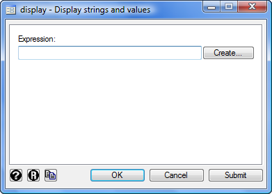
It’s known as Stata’s expression builder. You may get to it from the show dialog (Knowledge->Different Utilities->Hand Calculator)
Within the dialog, click on the Create button to convey up the builder. Actually, it doesn’t seem like a lot:

I wish to present you find out how to use this expression builder; in the event you’ll follow me, it’ll be value your time.
Let’s begin over once more and assume you’re within the midst of an evaluation, say,
. sysuse auto, clear
. regress worth mpg size
Subsequent invoke the expression builder by knocking down the menu Knowledge->Different Utilities->Hand Calculator. Click on Create. It seems like this:
Now click on on the tree node icon (+) in entrance of “Estimation outcomes” after which scroll right down to see what’s beneath. You’ll see

Click on on Scalars:

The center field now incorporates the scalars saved in e(). N occurs to be highlighted, however you would click on on any of the scalars. If you happen to look beneath the 2 packing containers, you see the worth of the e() scalar chosen in addition to its worth and a brief description. e(N) is 74 and is the “variety of observations”.
It really works the identical means for all the opposite classes within the field on the left: Operators, Capabilities, Variables, Coefficients, Estimation outcomes, Returned outcomes, System parameters, Matrices, Macros, Scalars, Notes, and Traits. You merely click on on the tree node icon (+), and the class expands to point out what is on the market.
You’ve now mastered the expression builder!
Let’s attempt it out.
Say you wish to confirm that the p-value of the coefficient on mpg is accurately calculated by regress–which reviews 0.052–or extra possible, you wish to confirm that you understand how it was calculated. You assume the method is

or, as an expression in Stata,
2*ttail(e(df_r), abs(_b[mpg]/_se[mpg]))
However I’m leaping forward. It’s possible you’ll not keep in mind that _b[mpg] is the coefficient on variable mpg, or that _se[mpg] is its corresponding customary error, or that abs() is Stata’s absolute worth perform, or that e(df_r) is the residual levels of freedom from the regression, or that ttail() is Stata’s Pupil’s t distribution perform. We are able to construct the above expression utilizing the builder as a result of all of the parts could be accessed by way of the builder. The ttail() and abs() capabilities are within the Capabilities class, the e(df_r) scalar is within the Estimation outcomes class, and _b[mpg] and _se[mpg] are within the Coefficients class.

What’s good concerning the builder is that not solely are the merchandise names listed but in addition a definition, syntax, and worth are displayed once you click on on an merchandise. Having all this data in a single place makes constructing a posh expression a lot simpler.
One other instance of when the expression builder turns out to be useful is when computing intraclass correlations after xtmixed. Think about a easy two-level mannequin from Instance 1 in [XT] xtmixed, which fashions weight trajectories of 48 pigs from 9 successive weeks:
. use http://www.stata-press.com/information/r12/pig
. xtmixed weight week || id:, variance
The intraclass correlation is a nonlinear perform of variance parts. On this instance, the (residual) intraclass correlation is the ratio of the between-pig variance, var(_cons), to the full variance, between-pig variance plus residual (within-pig) variance, or var(_cons) + var(residual).
The xtmixed command doesn’t retailer the estimates of variance parts instantly. As a substitute, it shops them as log customary deviations in e(b) such that _b[lns1_1_1:_cons] is the estimated log of between-pig customary deviation, and _b[lnsig_e:_cons] is the estimated log of residual (within-pig) customary deviation. So to compute the intraclass correlation, we should first rework log customary deviations to variances:
exp(2*_b[lns1_1_1:_cons])
exp(2*_b[lnsig_e:_cons])
The ultimate expression for the intraclass correlation is then
exp(2*_b[lns1_1_1:_cons]) / (exp(2*_b[lns1_1_1:_cons])+exp(2*_b[lnsig_e:_cons]))
The issue is that few individuals keep in mind that _b[lns1_1_1:_cons] is the estimated log of between-pig customary deviation. The few who do definitely don’t wish to kind it. So use the expression builder as we do beneath:

On this case, we’re utilizing the expression builder accessed from Stata’s nlcom dialog, which reviews estimated nonlinear mixtures together with their customary errors. As soon as we press OK right here and within the nlcom dialog, we’ll see
. nlcom (exp(2*_b[lns1_1_1:_cons])/(exp(2*_b[lns1_1_1:_cons])+exp(2*_b[lnsig_e:_cons])))

  _nl_1:  exp(2*_b[lns1_1_1:_cons])/(exp(2*_b[lns1_1_1:_cons])+exp(2*_b[lnsig_e:_cons]))

------------------------------------------------------------------------------
      weight |      Coef.   Std. Err.      z    P>|z|     [95% Conf. Interval]
-------------+----------------------------------------------------------------
       _nl_1 |   .7717142   .0393959    19.59   0.000     .6944996    .8489288
------------------------------------------------------------------------------
The above might simply be prolonged to computing various kinds of intraclass correlations arising in higher-level random-effects fashions. Using the expression builder for that turns into much more useful.