

(newcommand{mub}{{boldsymbol{mu}}}
newcommand{eb}{{boldsymbol{e}}}
newcommand{betab}{boldsymbol{beta}})Utilized time-series researchers usually wish to examine the accuracy of a pair of competing forecasts. A well-liked statistic for forecast comparability is the imply squared forecast error (MSFE), a smaller worth of which means a greater forecast. Nonetheless, a proper check, comparable to Diebold and Mariano (1995), distinguishes whether or not the prevalence of 1 forecast is statistically vital or is solely because of sampling variability.
A associated check is the forecast encompassing check. This check is used to find out whether or not one of many forecasts encompasses all of the related data from the opposite. The ensuing check statistic could lead a researcher to both mix the 2 forecasts or drop the forecast that incorporates no extra data.
On this put up, I assemble a pair of one-step-ahead recursive forecasts for the change in inflation price from an autoregression mannequin (AR) and a vector autoregression mannequin (VAR). Primarily based on an train in Clark and McCracken (2001), I contemplate a bivariate VAR with modifications in inflation and unemployment price as dependent variables. I examine the forecasts utilizing MSFE, carry out exams of predictive accuracy and forecast encompassing to find out whether or not unemployment price is helpful in predicting inflation price. As a result of the VAR mannequin nests the AR mannequin, I assess the importance of the check statistic utilizing acceptable essential values offered in McCracken (2007) and Clark and McCracken (2001).
Forecasting strategies
Let (y_t) denote a collection we wish to forecast and (hat{y}_t) denote the (h)-step-ahead forecast of (y_t) at time (t). Out-of-sample forecasts are often computed with a set, rolling, or recursive window technique. In all of the strategies, an preliminary pattern of (T) observations is used to estimate the parameters of the mannequin. In a set window technique, estimation is carried out as soon as in a pattern of (T) observations and (h)-step-ahead forecasts are made based mostly on these estimates. In a rolling window technique, the dimensions of the estimation pattern is stored mounted. Nonetheless, estimation is carried out a number of occasions by incrementing the start and finish of the preliminary pattern by the identical quantity. Out-of-sample forecasts are computed after every estimation. A recursive window technique is just like a rolling window technique besides that the start time interval is held mounted whereas the the ending interval will increase.
I take advantage of the rolling prefix command with the recursive choice to generate recursive forecasts. rolling executes the command it prefixes on a window of observations and shops outcomes comparable to parameter estimates or different abstract statistics. Within the following part, I write instructions that match AR(2) and VAR(2) fashions, compute one-step-ahead forecasts, and return related statistics. I take advantage of these instructions with the rolling prefix and retailer the recursive forecasts in a brand new dataset.
Programming a command for the rolling prefix
In usinfl.dta, I’ve quarterly knowledge from 1948q1 to 2016q1 on the modifications in inflation price and the unemployment price obtained from the St. Louis FRED database. The primary mannequin is an AR(2) mannequin of change in inflation, which is given by
[
{tt dinflation}_{,,t} = beta_0 + beta_1 {tt dinflation}_{,,t-1} +
beta_2 {tt dinflation}_{,,t-2} + epsilon_t
]
the place (beta_0) is the intercept and (beta_1) and (beta_2) are the AR parameters. I generate recursive forecasts for these fashions starting in 2002q2. This means an preliminary window measurement of 218 observations from 1948q1 to 2002q1. The selection of the window measurement for computing forecasts in utilized analysis is unfair. See Rossi and Inoue (2012) for exams of predictive accuracy that’s sturdy to the selection of window measurement.
Within the following code block, I’ve a command labeled fcst_ar2.ado that estimates the parameters of an AR(2) mannequin utilizing regress and computes one-step-ahead forecasts.
program fcst_ar2, rclass
        syntax [if]

        qui tsset
        native timevar `r(timevar)'
        native first `r(tmin)'

        regress l(0/2).dinflation `if'
        summarize `timevar' if e(pattern)

        native final = `r(max)'-`first'+1
        native fcast = _b[_cons] + _b[l.dinflation]*     ///
                dinflation[`last'] + _b[l2.dinflation]* ///
                dinflation[`last'-1]

        return scalar fcast = `fcast'
        return scalar precise = dinflation[`last'+1]
        return scalar sqerror = (dinflation[`last'+1]-  ///
                `fcast')^2
finish
Line 1 defines the identify of the command and declares it to be rclass in order that I can return my ends in r() after executing the command. Line 2 defines the syntax for the command. I specify an if qualifier within the syntax in order that my command can establish the right observations when used with the rolling prefix. Traces 4–6 retailer the time variable and the start time index in my dataset as native macros timevar and first, respectively. Traces 8–9 use regress to suit an AR(2) mannequin and summarize the time variable within the pattern used for estimation. Line 11 shops the final time index within the native macro final. The one-step-ahead forecast for the AR(2) mannequin is
[
hat{y}_t = hat{beta}_0 + hat{beta}_1 {tt dinflation}_{,,t-1} + hat{beta}_2 {tt dinflation}_{,,t-2}
]
the place (hat{beta})’s are the estimated parameters. Traces 12–14 retailer the forecast in an area macro fcast. Traces 16–19 return the forecasted worth, precise worth, and the squared error in native macros fcast, precise, and sqerror, respectively. Line 20 specifies the tip of the command.
The second mannequin is a VAR(2) mannequin of change in inflation and unemployment price and is given by
[
begin{bmatrix} {tt dinflation}_{,,t}
{tt dunrate}_{,,t}
end{bmatrix}
= mub + {bf B}_1 begin{bmatrix} {tt
dinflation}_{,,t-1} {tt dunrate}_{,,t-1}
end{bmatrix}
+ {bf B}_2 begin{bmatrix}
{tt dinflation}_{,,t-2}
{tt dunrate}_{,,t-2}
end{bmatrix} + eb_t
]
the place (mub) is a (2times 1) vector of intercepts, ({bf B}_1) and ({bf B}_2) are (2times 2) matrices of parameters, and (eb_t) is a (2times 1) vector of IID errors with imply ({bf 0}) and covariance (boldsymbol{Sigma}).
Within the following code block, I’ve a command referred to as fcst_var2.ado that estimates the parameters of a VAR(2) mannequin utilizing var and computes one-step-ahead forecasts.
program fcst_var2, rclass

        syntax [if]

        quietly tsset
        native timevar `r(timevar)'
        native first `r(tmin)'

        var dinflation dunrate `if'
        summarize `timevar' if e(pattern)

        native final = `r(max)'-`first'+1
        native fcast = _b[dinflation:_cons] +             ///
                _b[dinflation:l.dinflation]*             ///
                dinflation[`last'] +                     ///
                _b[dinflation:l2.dinflation]*            ///
                dinflation[`last'-1] +                   ///
                _b[dinflation:l.dunrate]*dunrate[`last'] ///
                + _b[dinflation:l2.dunrate]*dunrate[`last'-1]

        return scalar fcast = `fcast'
        return scalar precise = dinflation[`last'+1]
        return scalar sqerror = (dinflation[`last'+1]-   ///
                `fcast')^2
finish
The construction of this command is just like the AR(2) I described earlier. The one-step-ahead forecast of dinflation equation for the VAR(2) mannequin is
[
hat{y}_t = hat{mu}_1 + hat{beta}_{1,11} {tt
dinflation}_{,,t-1} + hat{beta}_{1,12} {tt dunrate}_{,,t-1} +
hat{beta}_{2,11} {tt dinflation}_{,,t-2}
+ hat{beta}_{2,12}
{tt dunrate}_{,,t-2}
]
the place (hat{mu}_1) and (hat{beta})’s are the estimated parameters similar to the dinflation equation. Traces 13–19 retailer the one-step-ahead forecast in native macro fcast.
Recursive forecasts
I take advantage of the rolling prefix command with the command fcst_ar2. The squared errors, one-step-ahead forecast, and the precise values returned by fcst_ar2 are saved in variables named ar2_sqerror, ar2_fcst, and precise, respectively. I specify a window measurement of 218 and retailer the estimates within the dataset ar2.
. use usinfl, clear

. rolling ar2_sqerr=r(sqerror) ar2_fcast=r(fcast) precise=r(precise),
> window(218) recursive saving(ar2, change): fcst_ar2
(working fcst_ar2 on estimation pattern)

Rolling replications (56)
----+--- 1 ---+--- 2 ---+--- 3 ---+--- 4 ---+--- 5
..................................................    50
.....e
file ar2.dta saved
With a window measurement of 218, I’ve 55 usable observations which might be one-step-ahead forecasts. I do the identical with fcst_var2 beneath and retailer the estimates within the dataset var2.
. rolling var2_sqerr=r(sqerror) var2_fcast=r(fcast), window(218)
> recursive saving(var2, change): fcst_var2
(working fcst_var2 on estimation pattern)

Rolling replications (56)
----+--- 1 ---+--- 2 ---+--- 3 ---+--- 4 ---+--- 5
..................................................    50
.....e
file var2.dta saved
I merge the 2 datasets containing the forecasts and label the precise and forecast variables. I plot the precise versus the forecasts of dinflation obtained from an AR(2) and a VAR(2) mannequin respectively.
. use ar2, clear
(rolling: fcst_ar2)
. quietly merge 1:1 finish utilizing var2
. tsset finish
time variable: finish, 2002q2 to 2016q1
delta: 1 quarter
. label var finish "Quarterly date"
. label var precise "Change in inflation"
. label var ar2_fcast "Forecasts from AR(2)"
. label var var2_fcast "Forecasts from VAR(2)"
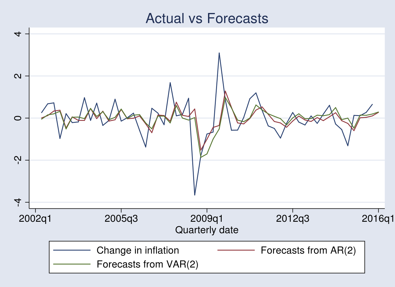
. tsline precise ar2_fcast var2_fcast, title("Precise vs Forecasts")
Each fashions produce forecasts that monitor the precise change in inflation. Nonetheless, the efficiency of 1 forecast from the opposite is indistinguishable from the determine above.
Evaluating MSFE
A well-liked statistic used to match out-of-sample forecasts is the MSFE. I take advantage of the imply command to compute this.
. imply ar2_sqerr var2_sqerr

Imply estimation                   Variety of obs   =         55

--------------------------------------------------------------
             |       Imply   Std. Err.     [95% Conf. Interval]
-------------+------------------------------------------------
   ar2_sqerr |   .9210348   .3674181      .1844059    1.657664
  var2_sqerr |   .9040102   .3377726      .2268169    1.581203
--------------------------------------------------------------
The MSFE of the forecasts produced by the VAR(2) mannequin is barely smaller than that of the AR(2) mannequin. This comparability, nonetheless, is predicated on a single pattern and doesn’t replicate the predictive efficiency within the inhabitants.
Take a look at for equal predictive accuracy
McCracken (2007) gives check statistics to check the predictive accuracy of forecasts generated by a pair of nested parametric fashions. Beneath the null speculation, the anticipated lack of the pair of forecasts is similar. Beneath the choice, the anticipated lack of the larger mannequin is lower than that of the one it nests. Within the present software, the null and the choice speculation are as follows
[
H_o: E[L_{t+1}(betab_1)] = E[L_{t+1}(betab_2)] quad mbox{vs} quad
H_a: E[L_{t+1}(betab_1)] > E[L_{t+1}(betab_2)]
]
the place (L_{t+1}(cdot)) denotes a squared error loss. (betab_1) and (betab_2) are the parameter vectors of the AR(2) and VAR(2) fashions, respectively.
I assemble two check statistics, which McCracken labels as OOS-F and OOS-T for out-of-sample F and t exams. The OOS-T statistic is predicated on Diebold and Mariano (1995). The limiting distribution of each check statistics is nonstandard. The OOS-F and OOS-T check statistics are as follows
[
mathrm{OOS-F} = P left[ frac{mathrm{MSFE}_1(hat{beta}_1) –
mathrm{MSFE}_2(hat{beta}_2)}{mathrm{MSFE}_2(hat{beta}_2)}right]
mathrm{OOS-T} = hat{omega}^{-0.5} left[ mathrm{MSFE}_1(hat{beta}_1) –
mathrm{MSFE}_2(hat{beta}_2)right]
]
the place (P) is the variety of out-of-sample observations and (mathrm{MSFE}_1(cdot)) and (mathrm{MSFE}_2(cdot)) are the imply squared forecast error of the AR(2) and VAR(2) fashions, respectively. (hat{omega}) denotes a constant estimate of the asymptotic variance of the imply of the squared-error loss differential. I compute the OOS-F statistic beneath:
. quietly imply ar2_sqerr var2_sqerr

. native msfe_ar2 = _b[ar2_sqerr]

. native msfe_var2 = _b[var2_sqerr]

. native P = 55

. show "OOS-F: " `P'*(`msfe_ar2'-`msfe_var2')/`msfe_var2'
OOS-F: 1.0357811
The corresponding 95% essential worth from desk 4 (utilizing (pi=0.2) and (k_2=2)) in McCracken (2007) is 1.453. The OOS-F fails to reject the null speculation, implying that the forecasts from the AR(2) and VAR(2) have comparable predictive accuracy.
To compute the OOS-T statistic, I first estimate (hat{omega}) by utilizing the heteroskedasticity and autocorrelation constant (HAC) normal error from a regression of squared error loss differential on a continuing.
. generate ld = ar2_sqerr-var2_sqerr
(1 lacking worth generated)

. gmm (ld-{_cons}), vce(hac nwest 4) nolog
notice: 1 lacking worth returned for equation 1 at preliminary values

Remaining GMM criterion Q(b) =  4.41e-35

notice: mannequin is strictly recognized

GMM estimation

Variety of parameters =   1
Variety of moments    =   1
Preliminary weight matrix: Unadjusted              Variety of obs   =         55
GMM weight matrix:     HAC Bartlett 4

---------------------------------------------------------------------------
          |                 HAC
          |      Coef.   Std. Err.      z    P>|z|     [95% Conf. Interval]
----------+----------------------------------------------------------------
   /_cons |   .0170247   .0512158     0.33   0.740    -.0833564    .1174057
---------------------------------------------------------------------------
HAC normal errors based mostly on Bartlett kernel with 4 lags.
Devices for equation 1: _cons

. show "OOS-T: " (`msfe_ar2'-`msfe_var2')/_se[_cons]
OOS-T: .33241066
The corresponding 95% essential worth from desk 1 in McCracken (2007) is 1.140. The OOS-T additionally fails to reject the null speculation, implying that the forecasts from the AR(2) and VAR(2) have comparable predictive accuracy.
Take a look at for forecast encompassing
Beneath the null speculation, forecasts from mannequin 1 embody that from mannequin 2; thus forecasts from the latter mannequin include no extra data. Beneath the choice speculation, forecast from mannequin 2 include extra data than that from mannequin 1. The brand new encompassing check statistic labeled as ENC-New in Clark and McCracken (2001) is given by
[
mathrm{ENC-New} = P left[ frac{mathrm{MSFE}_1(hat{beta}_1) –
sum_{t=1}^Phat{e}_{1,t+1}hat{e}_{2,t+1}/P}{mathrm{MSFE}_2(hat{beta}_2)}right]
]
the place (hat{e}_{1,t+1}) and (hat{e}_{2,t+1}) are one-step-ahead forecast errors. I compute the ENC-New statistic beneath:
. generate err_p = sqrt(ar2_sqerr*var2_sqerr)
(1 lacking worth generated)

. generate numer = ar2_sqerr-err_p
(1 lacking worth generated)

. quietly summarize numer

. show "ENC-NEW: " `P'*(r(imply)/`msfe_var2')
ENC-NEW: 1.3818277
The corresponding 95% essential worth from desk 1 in Clark and McCracken (2001) is 1.028. The ENC-New check rejects the null speculation, implying that the forecasts from the AR(2) don’t embody the VAR(2) forecasts. In different phrases, unemployment price is helpful for forecasting inflation price.
The failure to reject the null speculation by the OOS-F and OOS-T check could also be as a result of lack of energy of those exams in contrast with that of the ENC-New check.
Conclusion
On this put up, I used the rolling prefix command to generate out-of-sample recursive forecasts from an AR(2) of modifications in inflation and a VAR(2) mannequin of modifications in inflation and unemployment price. I then constructed check statistics for forecast accuracy and forecast encompassing to find out whether or not unemployment price is helpful for forecasting inflation price.
References
Clark, T. E., and M. W. McCracken. 2001. Checks of equal forecast accuracy and encompassing for nested fashions. Journal of Econometrics 105: 85–110.
Diebold, F. X., and R. S. Mariano. 1995. Evaluating predictive accuracy. Journal of Enterprise and Financial Statistics 13: 253–263.
McCracken, M. W. 2007. Aymptotics for out of pattern exams of Granger causality. Journal of Econometrics 140: 719–752.
Rossi, B., and A. Inoue. 2012. Out-of-sample forecast exams sturdy to the selection of window measurement. Journal of Enterprise and Financial Statistics 30: 432–453.