A number of Brokers Auditing Your Callaway and Sant’Anna Diff-in-Diff (Half 3)

Final week I had Claude implement a “multi-analyst design” throughout 5 Callaway and Sant’Anna packages (2 in python, 1 in R, 2 in Stata) on a hard and fast dataset, a common baseline, ~20 covariates to select from for satisfying conditional parallel tendencies, and the identical goal parameter. You’ll find that right here:

However in that submit, I didn’t end reporting it. So I filmed myself going by means of the “lovely deck” it produced. And on this substack, I’ll clarify in phrases what it discovered, however the gist is that there was surprisingly great amount of variation between packages but additionally inside packages within the variation within the outcomes throughout 15 complete runs. Right here’s the video:

And I simply needed to once more thank everybody for supporting the substack. It has been very nice to put in writing about Claude Code these final two and a half months since my first submit December thirteenth, 2025. I’ve been studying so much over these 28 posts (!). I actually take pleasure in making an attempt to determine how one can use Claude Code for “sensible empirical analysis” — on a regular basis, run of the mill, sort of utilized stuff. And it’s been a bit like making an attempt to experience a wild stallion. In order that’s been enjoyable too as I wanted the thrill.

In case you are a paying subscriber — thanks. I admire your assist. And in the event you aren’t a paying subscriber, keep in mind that the Claude Code posts are all free for round 4 days, however then they go behind the paywall. The extra typical non-AI posts are often randomized behind the paywall, however as Claude Code is a brand new factor, and I need to assist folks see its worth for sensible empirical work, I submit these without cost, they sit open for 4 days, after which all of them go behind the paywall. Hopefully that’ll be sufficient that can assist you see what’s occurring. However maybe that is the day you are feeling like changing into a paying subscriber! At solely $5/mo, it’s a deal!

Breaking down what I discovered

So in the event you return to that earlier entry (half 2 particularly), you’ll get the breakdown of what this experiment is about. And if you wish to watch the video, that’ll assist too. However let’s now dig in. It’s also possible to evaluation the “lovely deck” too if you’d like.

There’s two “goal parameters” on this train of be aware. The primary are occasion research which combination as much as all relative time durations and if cohorts differ in measurement, and the weights are proportional to cohort measurement, then it’s a weighted common utilizing cohort measurement as weighting on the acceptable locations. I additionally am balancing the occasion research which suggests the identical cohorts seem in all l=-4 to l=+4 relative time durations. Due to this fact no compositional change in who’s and isn’t in every of those occasion research plots.

In order that’s one of many parameters. And the opposite is I’ll then take a easy weighted common over l=0 to l=+4 (thus every weight there’s 0.2 off an already weighted common that used cohort measurement as weights for the occasion research). And due to this fact in these, we’ll see each.

Forest plot of common level estimates

The primary although is a forest plot of the 15 estimates throughout all 5 language-packages. And that is fairly fascinating as a result of discover that whereas all of them are constructive results, 2 of them have big confidence intervals, and considered one of them (python’s diff-diff run 1) is massive and statistically totally different, not simply from zero, however from 11 of the others. The remainder are round 0.4 on common.

Occasion research

Listed below are the person level estimates from the occasion research all laid on prime of one another:

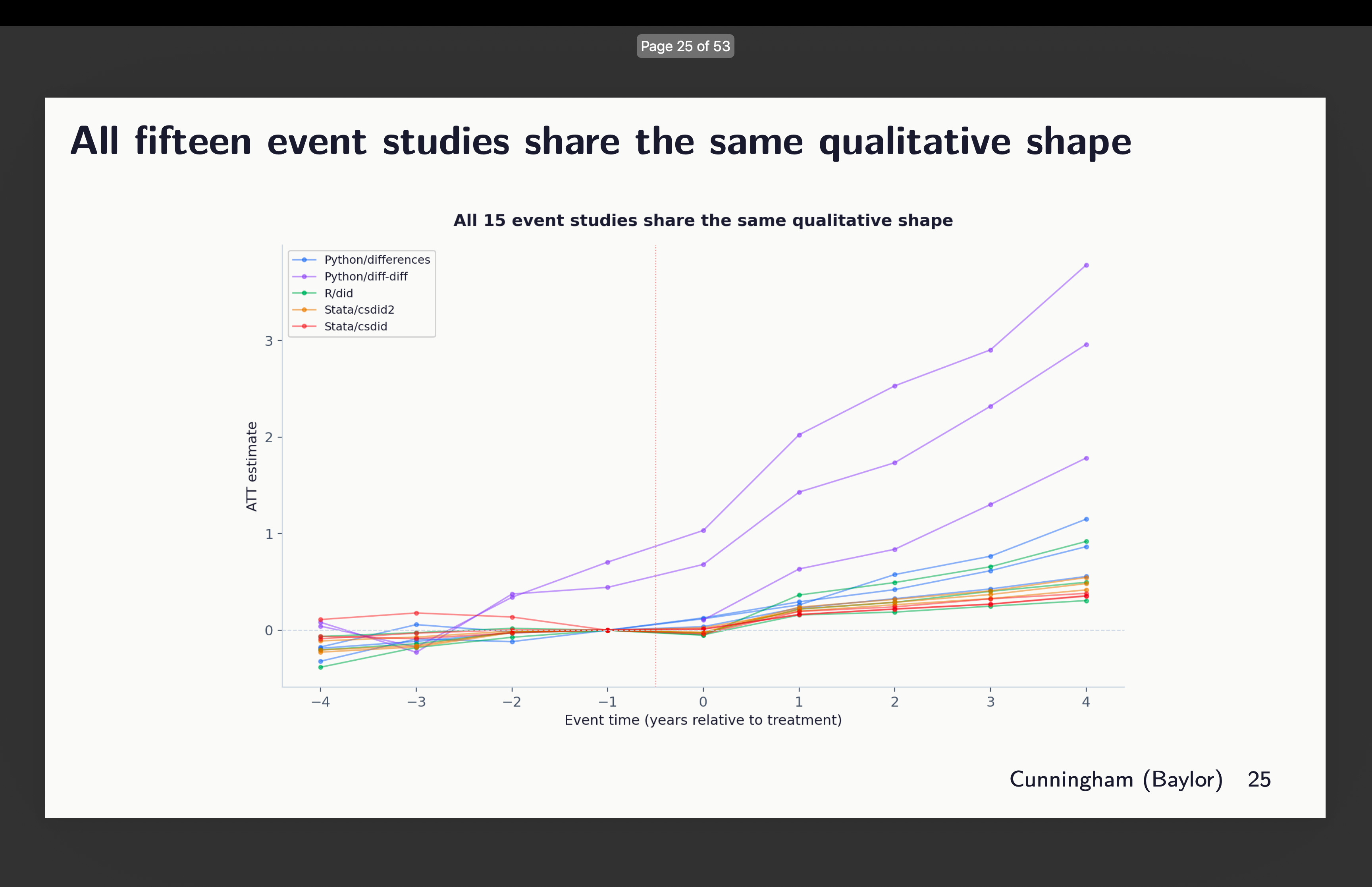
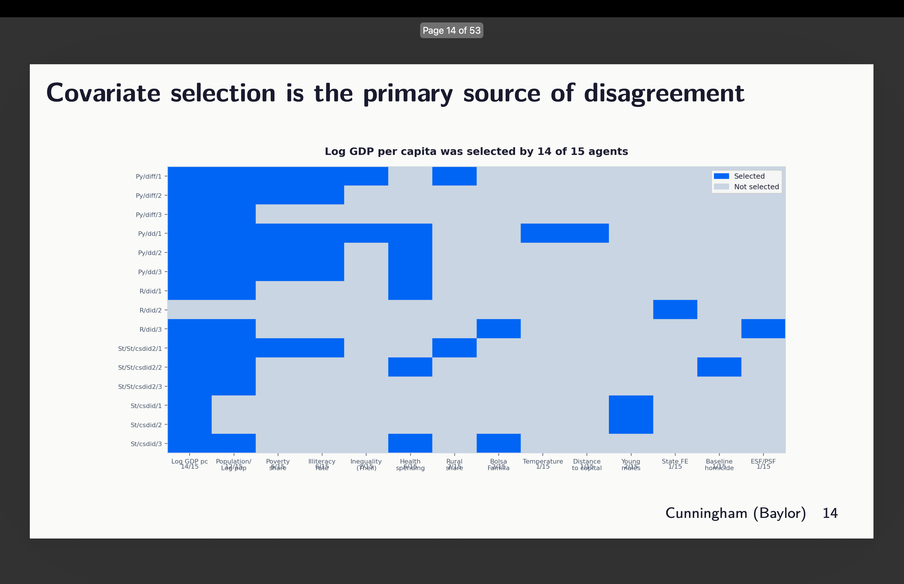
So you’ll be able to see right here some odd issues. First, it seems that two of our runs didn’t obey orders to make use of the common baseline. Discover that there are two graphs rising from round l=-3. That’s the python package deal diff-diff. I’ll present you that in a second. The others are similar-ish, however they bear taking a look at extra intently. I’ll focus on them so as. However earlier than I do, let’s simply remind ourselves which runs selected which covariates with this graphic:

Python’s variations packages

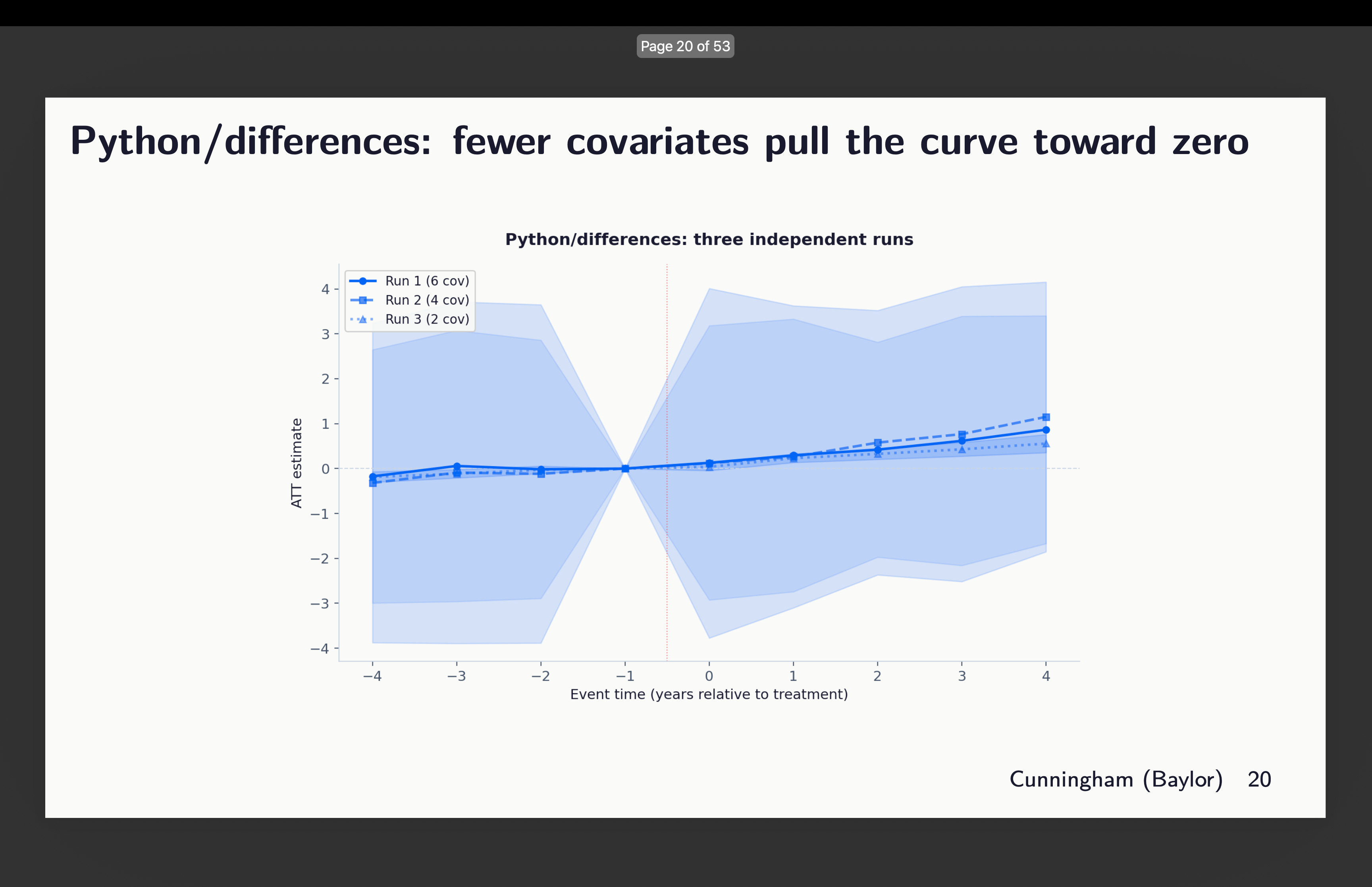
First I regarded on the three runs from variations written in python. Now right here’s an odd factor although — why are these 95% confidence intervals huge? Look how they vary just about from -4 to +4. Why is that? In order that’s one thing I need to higher perceive, however for now discover simply that they do, and that the variations inside this are covariates of two, 4 and 6 chosen. You may see above which of them that was.

Python’s diff-diff

Subsequent is Isaac Gerberg’s bold diff-diff package deal which he has been constructing all this yr. What did we discover there? You may evaluation the covariates chosen above to interpret these outcomes.

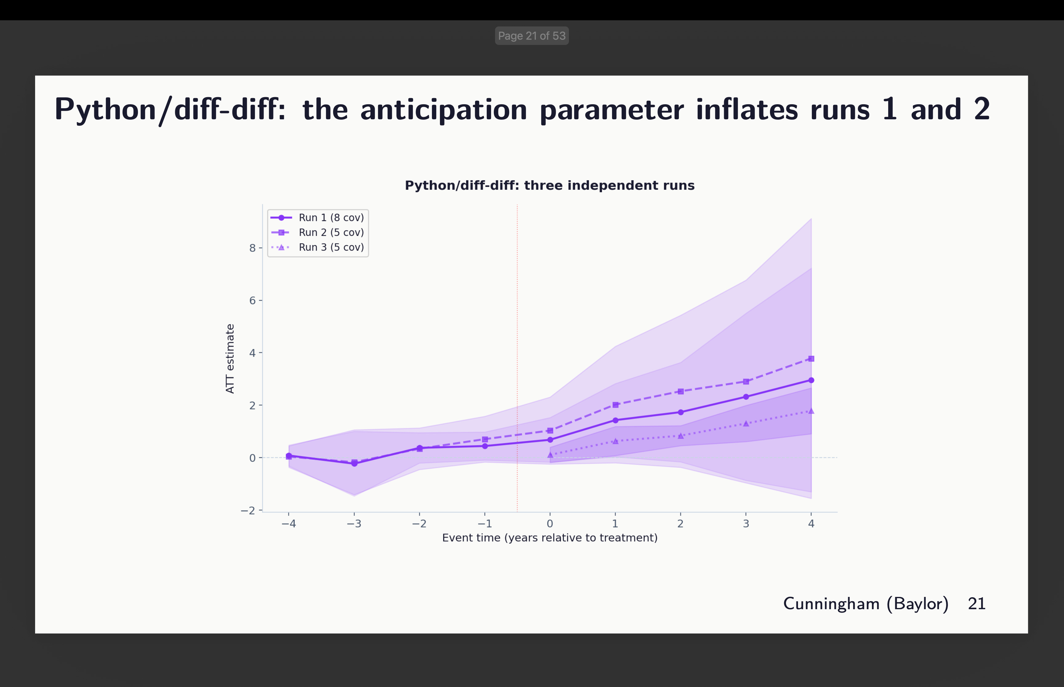
Okay, effectively this can be a unusual one. Why? As a result of Claude actually refused to do what I stated right here which was use g-1 because the common baseline. In two of them, it used g-5 because the baseline. And in considered one of them, it did use g-1, however didn’t estimate the pre-treatment coefficients.

It is a good place to simply pause and say one thing about utilizing g-5 as your baseline. That’s completely discover to do. However be aware that while you do it, whereas your goal parameter stays the identical — we’re in every of those estimating aggregated ATT(g,l) parameters — the parallel tendencies assumption is altering. And that’s as a result of in Callaway and Sant’Anna, therapy results are estimated utilizing whichever baseline you choose and are all the time “lengthy variations” too. The pre-treatment coefficients could be both lengthy or quick variations, however the therapy results can solely be lengthy variations. Which implies the parallel tendencies assumption is all the time lengthy variations too. In reality when doubtful, simply keep in mind that in CS, no matter is the outline of the traits of your ATT(g,t) goal parameter (e.g., covariates, weights) carries over to your parallel tendencies assumption too, solely it’s then a diff-in-diff easy 2×2 estimated as lengthy variations within the potential final result, Y(0), itself.

Which is to say that whereas the goal parameters are the identical right here, the parallel tendencies assumption is shifting round. And that’s discover when you have balanced pre-trends, however right here we don’t, which is itself fascinating, and that as a consequence the python variations packages is discovering a lot bigger coefficients in submit and pre than others do. It doesn’t look like an error a lot as Claude didn’t perceive the documentation and couldn’t due to this fact determine how one can implement what I requested. That is one thing I’m engaged on subsequent.

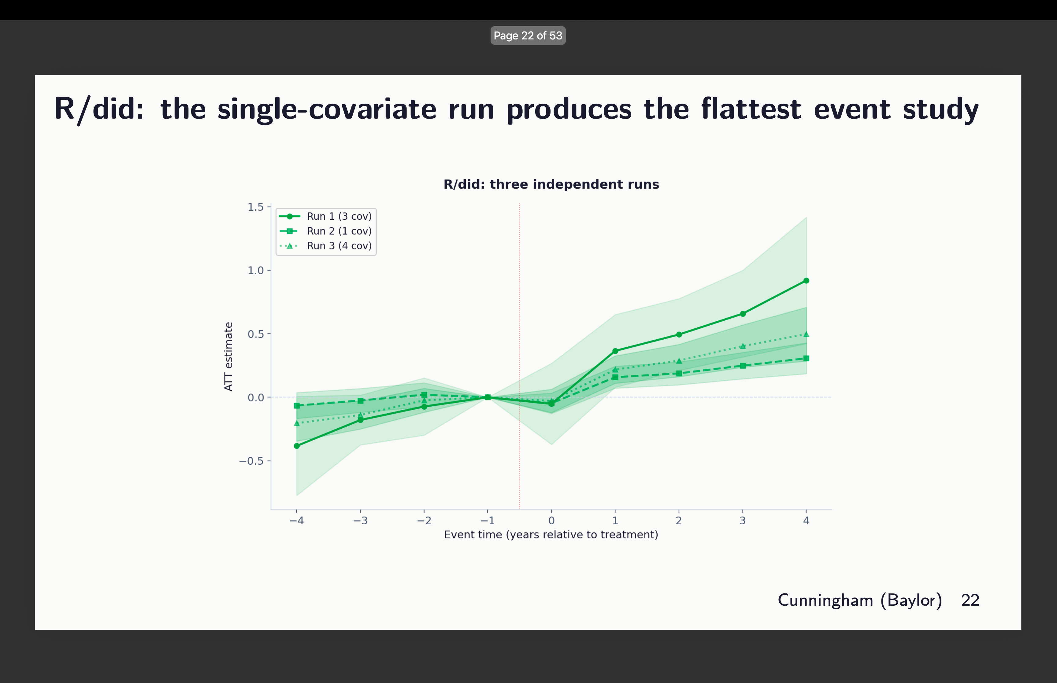
Authentic R did

Subsequent I regarded on the occasion research plots for R’s did. And this one once more selected totally different units of covariates, however right here’s what worrying — the one which selected 3 (out of 21 covariates thoughts you) reveals indicators of tendencies, whereas the one with only one covariate seems flatter. So which is it? Which of these three do you assume satisfies conditional parallel tendencies?

Give it some thought for a second. What number of papers have you ever ever seen that reveals variation in estimates throughout covariate choice and package deal choice? How about none? What do you usually see as a substitute? You extra typically see robustness to which diff-in-diff estimator — the well-known “all of the diff-in-diff plotted on prime of one another” graphic. However you don’t ever see somebody exploring covariates or packages. Shifting on.

Stata: csdid2 and csdid

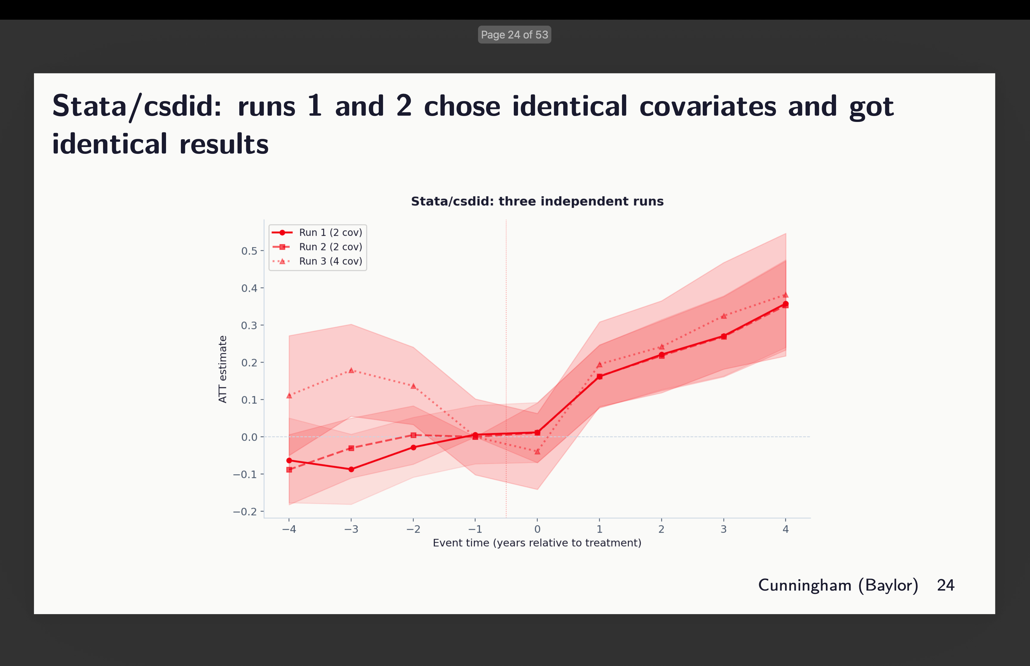
And at last, I have a look at the 2 Stata packages: the generally used csdid (out there from ssc) and csdid2 (now archived). I included it as a result of Claude selected it, so I included it as a result of I feel folks might need to use it because it’s quick. Although in our case it was not as quick as R. There’s not so much to report besides to say that relying on which and what number of covariates to situation on, we would see indicators of rising tendencies — some extra worrisome than others

After which I checked out csdid. Claude stated they selected similar covariates. But it surely’t not clear to me then why pre-trends are totally different. I didn’t dig into this as a result of I’m rerunning the entire thing now with 20 brokers per package deal (and yet one more further one) to get 120 estimates, after which I’ll dig into that. However right here’s that occasion research.

Variation Inside and Throughout Packages

Okay, so now that is the bizarre consequence. The extra covariates included, the bigger the purpose estimates altogether. You may see that right here, however discover that the majority of that is coming from the variation throughout packages which you’ll see in the event you look intently on the colours. That massive outlier on the far proper is definitely the python diff-diff one which used each 8 covariates (therefore why it’s up there), but additionally used g-5 as its baseline. And bear in mind due to slight rising tendencies within the pre-period, by the point it will get to the tip of the durations, it’s bought a head begin and is rising. That’s why it’s averaging out to 1.75.

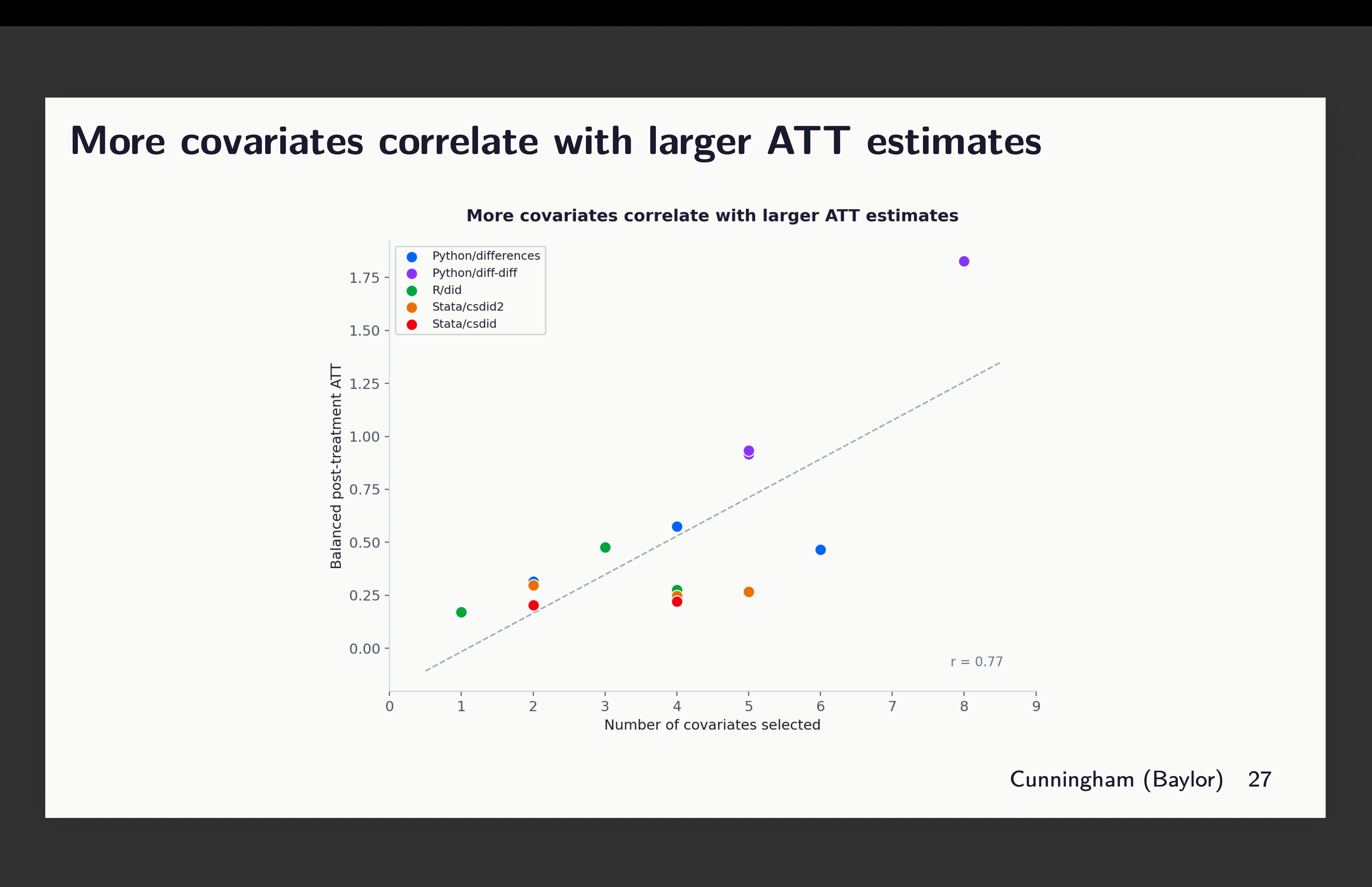
However even throwing out that outlier, you’ll be able to see nonetheless the correlation — the extra covariates included, the bigger the ATT estimate we discover, although all of those brokers use the identical dataset, technique, baseline, estimator and double strong, given solely the directions to “select covariates that fulfill parallel tendencies”. So just by choosing kind of covariates, you get bigger or smaller results alone.

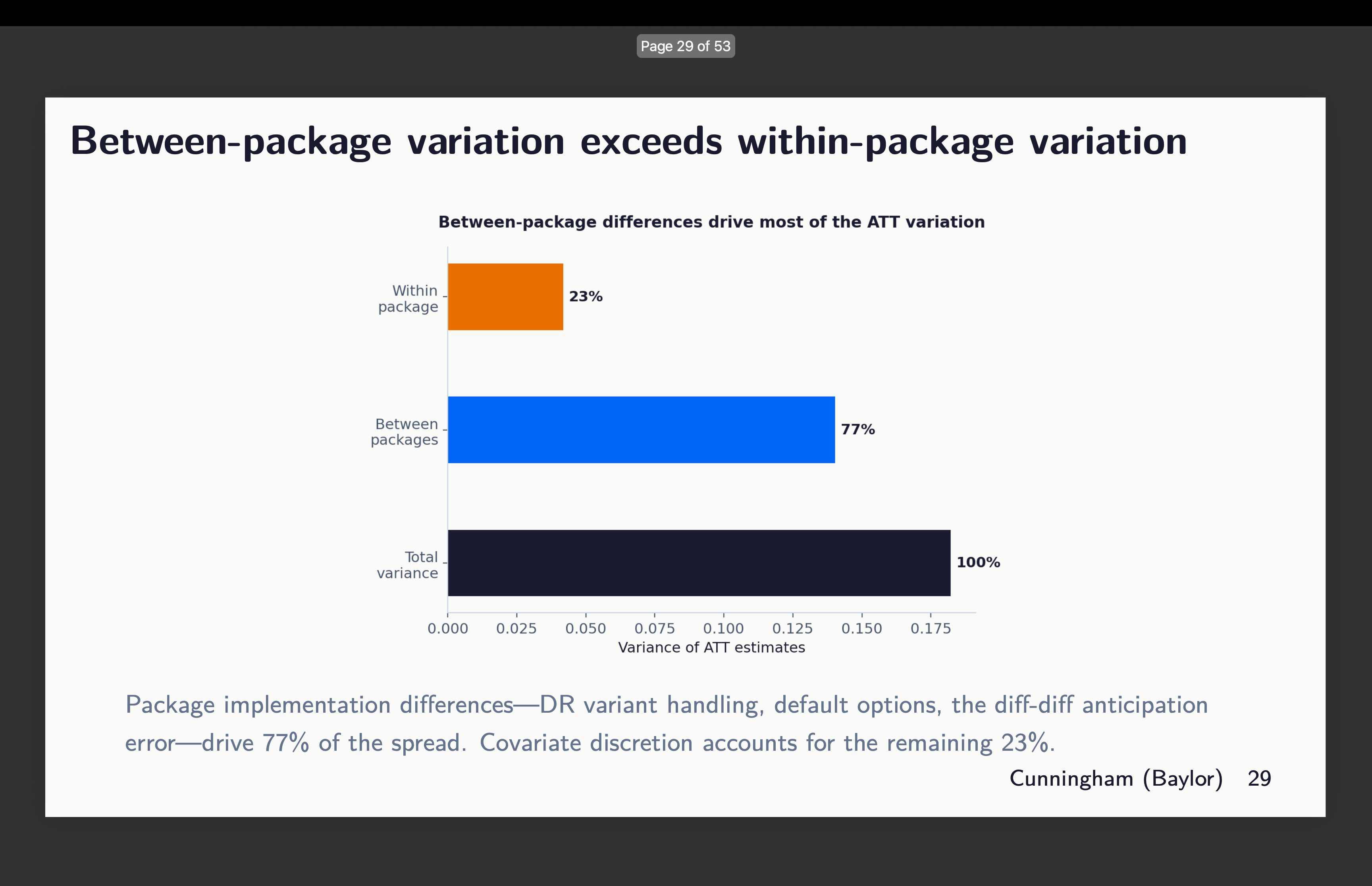
However then the opposite dimension the place there’s a variety of variation is the between packages. There may be variation inside too, however round 77% of it comes from the choice of which software program package deal to make use of. See right here:

Supporting Causes

Now I need you to assume again to the final time you noticed a chat utilizing diff-in-diff when the researcher listed covariates. Did they spend extra time explaining the estimator or did they spend extra time explaining the covariates and the rationale for every considered one of them? And did they ever point out which package deal they used? I wager good cash that talked extra in regards to the CS estimator and the assumptions than they did covariates or package deal, and doubtless didn’t point out the package deal as a result of why would they? Aren’t all of the packages giving the identical factor?

So I don’t know but the reply to the very last thing as a result of in no single case did any two brokers use the identical covariates throughout packages. So that’s nonetheless one thing I’ll look into however it’s not right here as a result of this isn’t about software program robustness; it’s about discretion on a single dimension — covariate choice. And I wager you not often have you ever heard somebody spend as a lot time explaining what and why these selected covariates as they did discuss in regards to the precise econometrics, proper? The brokers have been instructed to elucidate their rationale and right here it was:5

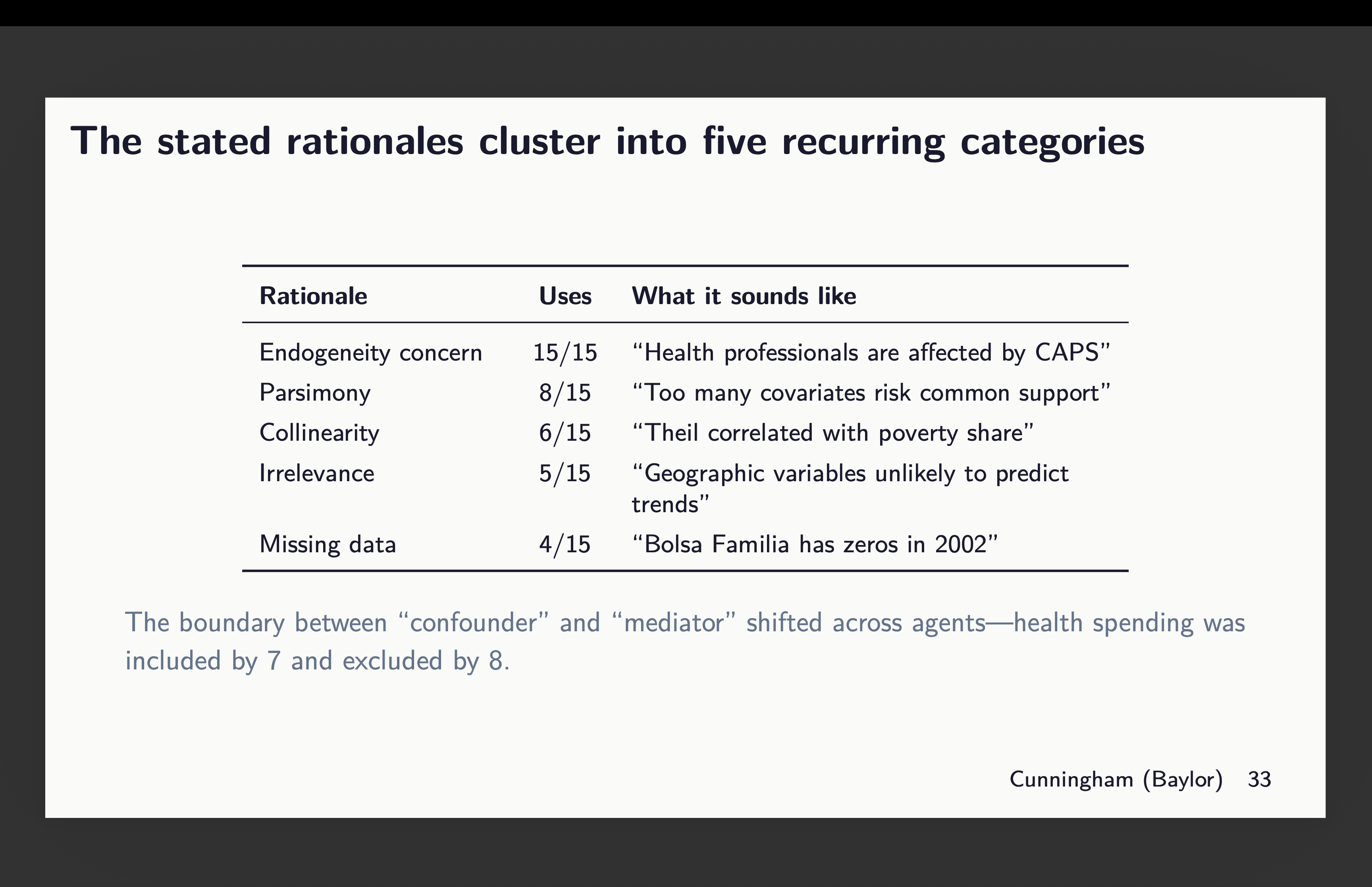
There’s mainly causes they gave for covariate choice they usually’re listed above. Now I need you to think about for a minute you’re in a chat, and somebody does clarify their alternative. Would you object to their rationalization? In all probability not. You’re extra more likely to object to the estimator (“why are you utilizing TWFE?”) than you’re to the covariates, and but covariates are driving variation in estimates on this experiment. So simply let that sink in.

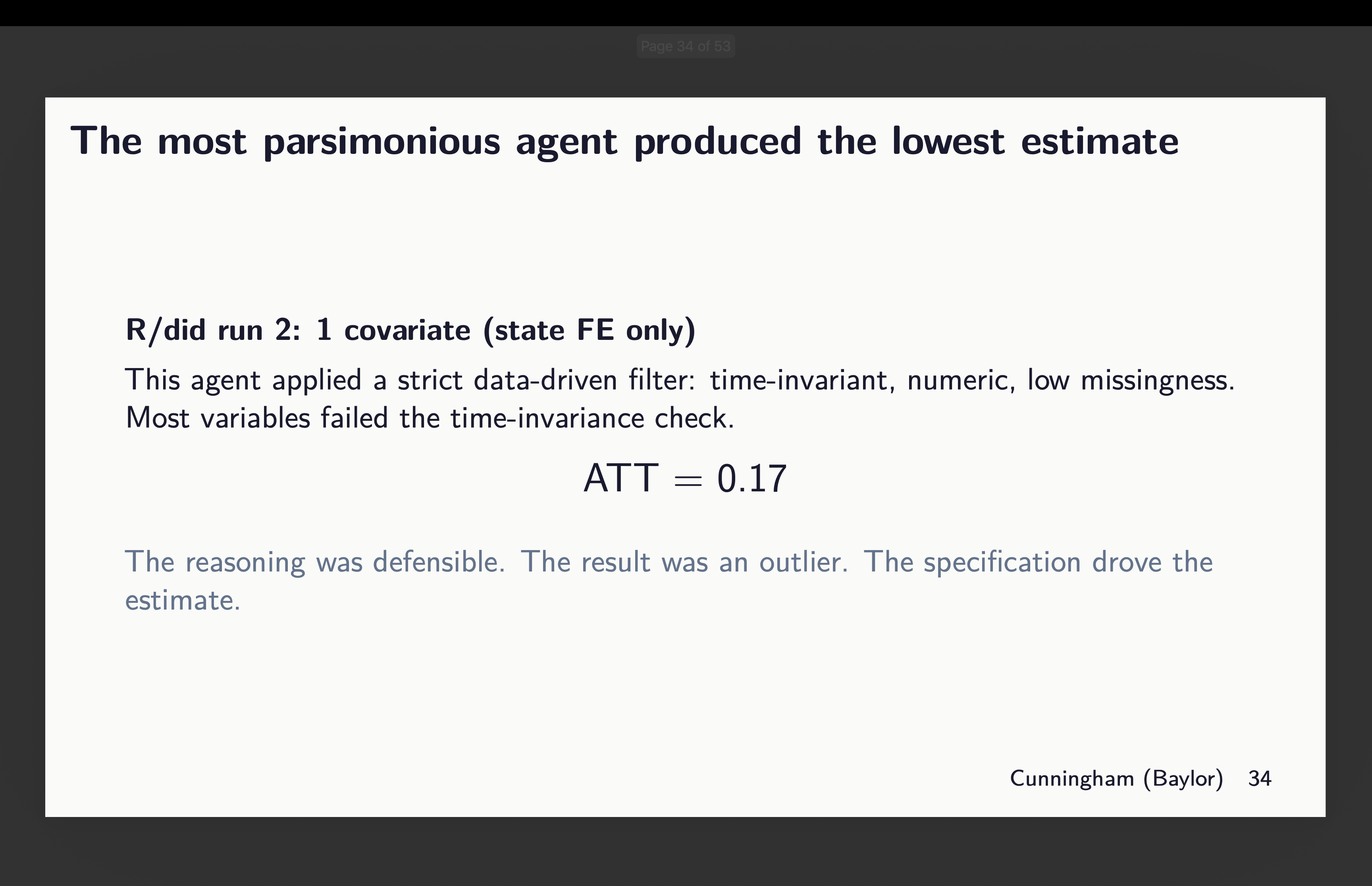
How massive of a distinction? Considered one of them R brokers utilizing did selected solely state mounted results (bear in mind that is municipality information so there’s variation inside a state mounted impact for estimating that first stage). For it, the purpose estimate was 0.17.

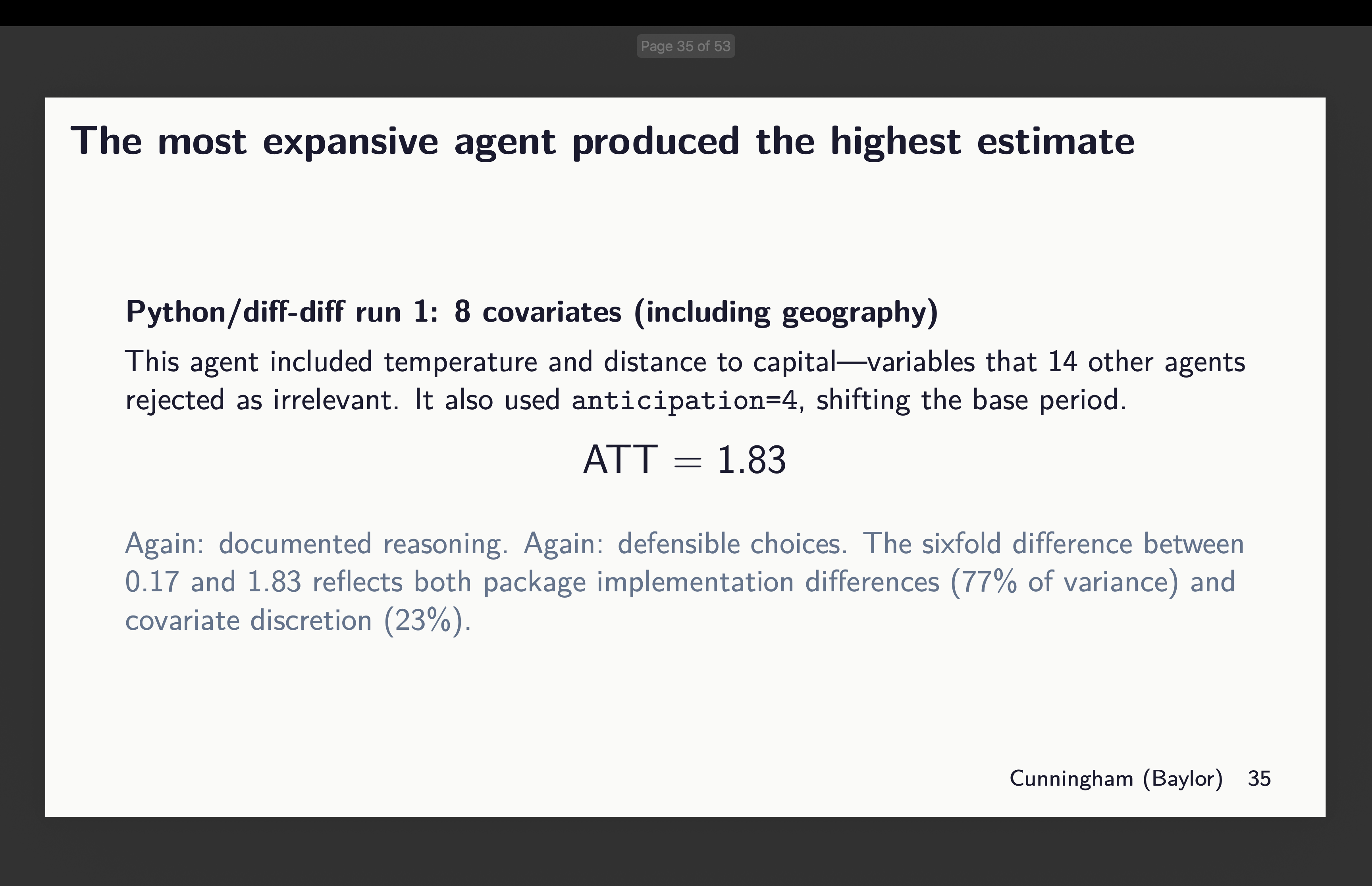
However now have a look at the agent given python’s diff-diff who selected 8 covariates. Its estimate is nearly 11 occasions bigger. And each documented their causes, and arguably all of them have been defensible. I don’t know why Claude stated this can be a six fold enhance when 1.83/0.17=10.765 however no matter.

How massive are the “non-standard errors”?

Now to the perfect half. Given now we have 15 estimates, aggregated into that easy ATT, weighted over all post-treatment ATT(g,l) from 0 to 4, what can we do to measure the uncertainty on this parameter. Let’s pause for a second and evaluation what the usual error means within the first place.

Below repeated sampling, you get a sequence of hypothetical samples from which you’d run CS on every one, after which while you have a look at the distribution of these estimates, you may have a random variable that varies in accordance with that fashions software to its personal i.i.d. drawn pattern. And the usual deviation in that sampling distribution is what our normal errors are supposed to seize. Within the regular distribution, 95% of chance as a single unit is inside roughly 2 normal deviations from the imply. And thus the p-value relies on the sampling distribution of the t-statistic – what p.c of t-statistics are greater than 1.96?

Okay, however then what about if now we have a mounted pattern, mounted dataset, however solely permit for discretion in covariate choice and package deal? And we permit n to be 15, with 3 runs per package deal? Effectively that’s not what our normal errors are supposed to seize although that may have a distribution. And if it has a distribution, it has variance, imply and normal deviation. However I even have the usual error for every run, in addition to the purpose estimate.

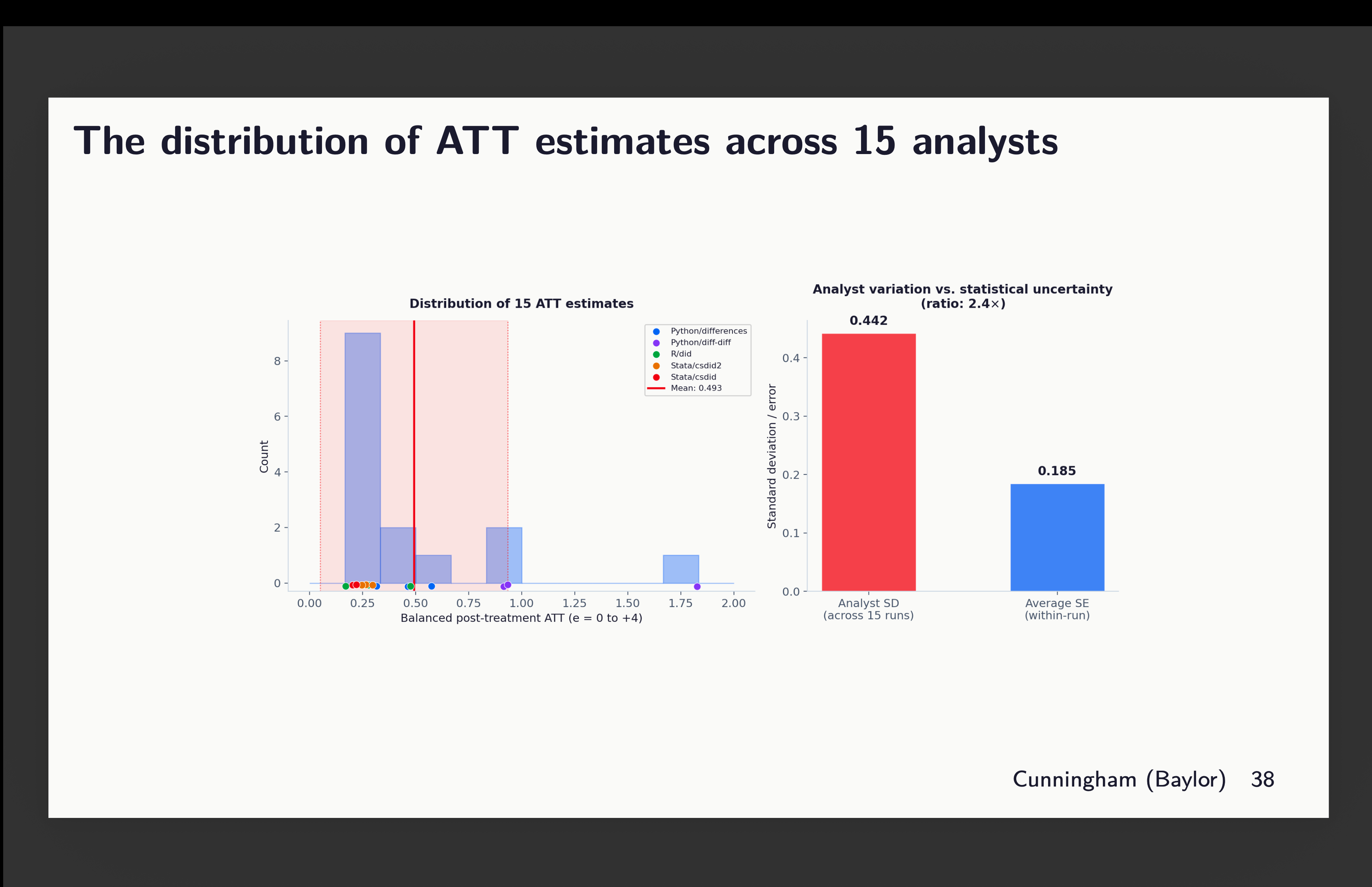
So what now we have right here is simply that however summarized. And verify this out. The purple field on the fitting is normal deviation throughout all my level estimates (together with the outlier from python diff-diff). And it’s a 0.442 normal deviation. But when I took the common of all 15 normal errors, that’s 0.185. And thus we get a 2.4 occasions bigger normal deviation in our 15 estimates than the common normal error for these 15 estimates.

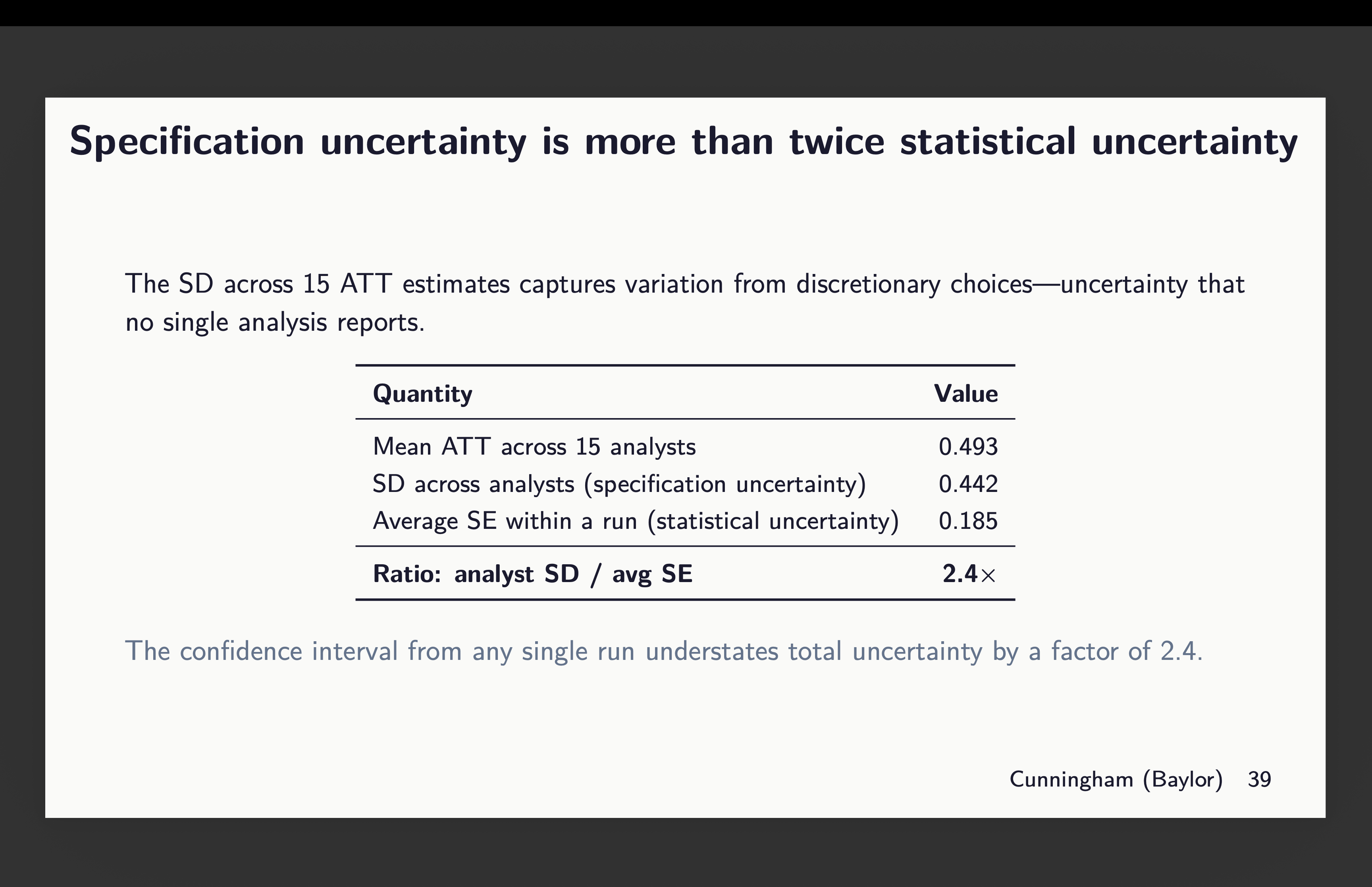
So now let that sink in. The usual errors we report are primarily based on repeated sampling. They’re designed to measure the statistical uncertainty related to the pattern and its correspondence to the inhabitants parameter. They’re not meant to measure uncertainty by which group labored on the mission. And but there’s that as a result of every group is choosing a special covariate mixture even with the identical dataset and even with the identical estimator and even with the identical experimental design.

So what’s subsequent?

So subsequent on the menu is just a few issues. They’re:

1. I’ll add within the doubleml package deal. It’s totally different structure, however it’s an inexpensive one to make use of. However in any other case it’s all 5 of those I reviewed right here plus a sixth.

2. I’ll enhance the runs from 3 to twenty brokers per package deal giving me 120 estimates when it’s completed.

3. I’ll proceed to make use of CS in all of those with the exception that doubleml might be totally different in its personal implementation, however that apart. Similar donor pool of covariates, similar not-yet-treated comparability group, similar common baseline (hopefully mounted this time for python’s diff-diff), and so on.

4. However now I’m going to permit for any covariates starting from none to all and any mixture it desires. The one rule is “select what satisfies conditional parallel tendencies”.

5. Every run will compute the standardized distinction in means on covariates utilizing baseline values averaged. It’s not ideally suited, however no matter — I would like this to not go on for 1,000,000 years.

6. And every will now have the choice to make use of IPW, regression adjustment or double strong, and if Stata, then whichever DR it desires.

So I’m simply going to be rigorously documenting this all and possibly on the finish of this, I’ll have discovered one thing, and in that case, hopefully all of us will be taught one thing. However I’m changing into increasingly of the opinion that we must be documenting this package deal and covariate choice much more rigorously than we’re. Packages all use the identical assumptions and are speculated to be figuring out the identical parameters. Their variations must be issues like pace and effectivity within the CPU. It shouldn’t be precise variations in numbers calculated. Customary errors might be totally different attributable to bootstrapping which makes use of random seeds, however the level estimates must be the identical given the identical covariates and modeling of these covariates within the first stage.

However the covariate choice and the way these are modeled — that’s the different two issues I’m making an attempt to pin down. So let’s see what we discover. I’ll have textual content by every agent explaining their causes and I could ship all 120 of these causes to openai to have gpt-4o-mini classify them. That could be overkill, however I really like doing that and so might do it once more.

That’s it! Keep tuned!