A New Approach of Least Squares

Should you’ve taken an introductory statistics or econometrics course, you almost certainly realized that the least squares regression line (widehat{alpha} + widehat{beta} x) minimizes the sum of squared vertical deviations by fixing the optimization drawback
[
max_{alpha, beta} sum_{i=1}^n (y_i – alpha – beta x_i)^2.
]
You most likely additionally realized that the answer is given by
[
widehat{alpha} = bar{y} – widehat{beta} bar{x}, quad
widehat{beta} = frac{sum_{i=1}^n (y_i – bar{y})(x_i – bar{x})}{sum_{i=1}^n (x_i – bar{x})^2} = frac{s_{xy}}{s_x^2}
]
In phrases: the regression slope equals the ratio of the covariance between peak and handspan to the variance of handspan, and the regression line passes by way of the pattern common values of peak and handspan. We are able to verify that every one of those formulation agree with what we calculated above utilizing lm()

b <- with(dat, cov(peak, handspan) / var(handspan))
a <- with(dat, imply(peak) - b * imply(handspan))
c(a, b)

## [1] 40.943127  1.266961

coef(lm(peak ~ handspan, dat))

## (Intercept)    handspan 
##   40.943127    1.266961

That is all completely appropriate, and a wholly cheap approach of wanting on the drawback. However I’d now prefer to recommend a fully completely different approach of taking a look at regression. Why hassle? The extra alternative ways we now have of understanding an thought or technique, the extra deeply we perceive the way it works, when it really works, and when it’s more likely to fail. So bear with me whereas I take you on what would possibly at first look like a poorly-motivated computational detour. I promise that there’s a payoff on the finish!

There’s a distinctive line that passes by way of any two distinct factors in a airplane. So right here’s a loopy thought: let’s type each distinctive pair of college students from my peak and handspan dataset. To know what I keep in mind, take into account a small subset of the info, name it take a look at

take a look at <- dat[1:3,]
take a look at

## # A tibble: 3 × 2
##   peak handspan
##        
## 1     73     22.5
## 2     65     17  
## 3     69     21

With three college students, there are three distinctive unordered pairs: ({1,2}, {1,3}, {2,3}). Corresponding to those three pairs are three line segments, one by way of every pair:

plot(peak ~ handspan, take a look at, pch = 20)
segments(x0 = c(17, 17, 21),     # FROM: x-coordinates
         y0 = c(65, 65, 69),     # FROM: y-coordinates
         x1 = c(21, 22.5, 22.5), # TO:   x-coordinates
         y1 = c(69, 73, 73),     # TO:   y-coordinates
         lty = 2)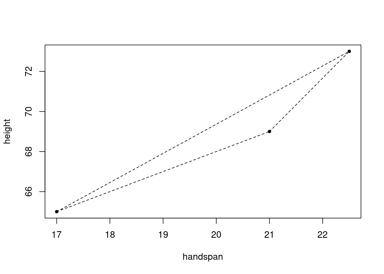

And related to every line phase is a slope

y_differences <- c(69 - 65, 73 - 65, 73 - 69)
x_differences <- c(21 - 17, 22.5 - 17, 22.5 - 21) 
slopes <- y_differences / x_differences
slopes

## [1] 1.000000 1.454545 2.666667

And right here’s my query for you: what, if something, is the connection between these three slopes and the slope of the regression line? Whereas it’s a bit foolish to run a regression with solely three observations, the outcomes are as follows:

coef(lm(peak ~ handspan, take a look at))

## (Intercept)    handspan 
##   41.556701    1.360825

The slope of the regression line doesn’t equal any of the three slopes we calculated above, nevertheless it does lie between them. This is smart: if the regression line had been steeper or much less steep than all three line segments from above, it couldn’t presumably reduce the sum of squared vertical deviations. Maybe the regression slope is the arithmetic imply of slopes? No such luck:

imply(slopes)

## [1] 1.707071

One thing fascinating is happening right here, nevertheless it’s not clear what. To be taught extra, it will be useful to play with greater than three factors. However doing this by hand can be extraordinarily tedious. Time to put in writing a perform!

The next perform generates all distinctive pairs of parts taken from a vector x and shops them in a matrix:

make_pairs <- perform(x) {
# Returns an information body whose rows comprise every unordered pair of parts of x
# i.e. all committees of two with members drawn from x
  n <- size(x)
  pair_indices <- combn(1:n, 2)
  matrix(x[c(pair_indices)], ncol = 2, byrow = TRUE)
}

For instance, making use of make_pairs() to the vector c(1, 2, 3, 4, 5) offers

make_pairs(1:5)

##       [,1] [,2]
##  [1,]    1    2
##  [2,]    1    3
##  [3,]    1    4
##  [4,]    1    5
##  [5,]    2    3
##  [6,]    2    4
##  [7,]    2    5
##  [8,]    3    4
##  [9,]    3    5
## [10,]    4    5

Discover that I’ve make_pairs() is constructed such that order doesn’t matter: we don’t distinguish between ((4,5)) and ((5,4)), for instance. This is smart for our instance: Alice and Bob denotes the identical pair of scholars as Bob and Alice.

To generate all attainable pairs of scholars from dat, we apply make_pairs() to dat$handspan and dat$peak individually after which mix the end result right into a single dataframe:

regression_pairs <- knowledge.body(make_pairs(dat$handspan), 
                               make_pairs(dat$peak))
head(regression_pairs)

##     X1   X2 X1.1 X2.1
## 1 22.5 17.0   73   65
## 2 22.5 21.0   73   69
## 3 22.5 25.5   73   71
## 4 22.5 25.0   73   78
## 5 22.5 20.0   73   68
## 6 22.5 20.5   73   75

The names are ugly, so let’s clear them up a bit. Handspan is our “x” variable and peak is our “y” variable, so we’ll check with the measurements from every pair as x1, x2, y1, y2

names(regression_pairs) <- c('x1', 'x2', 'y1', 'y2')
head(regression_pairs)

##     x1   x2 y1 y2
## 1 22.5 17.0 73 65
## 2 22.5 21.0 73 69
## 3 22.5 25.5 73 71
## 4 22.5 25.0 73 78
## 5 22.5 20.0 73 68
## 6 22.5 20.5 73 75

The 1 and 2 indices point out a specific scholar: in a given row x1 and y1 are the handspan and peak of the “first scholar” within the pair whereas x2 and y2 are the handspan and peak of the “second scholar.”
Every scholar seems many occasions within the regression_pairs dataframe. It’s because there are lots of pairs of scholars that embrace Alice: we are able to pair her up with every other scholar within the class. For that reason, regression_pairs has an incredible variety of rows, 52975 to be exact. That is the variety of methods to type a committee of measurement 2 from a set of 326 folks when order doesn’t matter:

select(326, 2)

## [1] 52975

Corresponding to every row of regression_pairs is a slope. We are able to calculate and summarize them as follows, utilizing the dplyr bundle from the tidyverse to make issues simpler to learn:

library(dplyr)
regression_pairs <- regression_pairs %>%
  mutate(slope = (y2 - y1) / (x2 - x1))
regression_pairs %>%
  pull(slope) %>%
  abstract

##    Min. 1st Qu.  Median    Imply third Qu.    Max.    NA's 
##    -Inf   0.000   1.333     NaN   2.667     Inf     419

The pattern imply slope is NaN, the minimal is -Inf, the utmost is Inf, and there are 419 lacking values. So what on earth does this imply? First issues first: the abbreviation NaN stands for “not a quantity.” That is R’s approach of expressing (0/0), and an NaN “counts” as a lacking worth:

0/0

## [1] NaN

is.na(0/0)

## [1] TRUE

In distinction, Inf and -Inf are R’s approach of expressing (pm infty). These do not depend as lacking values, they usually additionally come up when a quantity is simply too huge or too small in your laptop to signify:

c(-1/0, 1/0, exp(9999999), -exp(9999999))

## [1] -Inf  Inf  Inf -Inf

is.na(c(Inf, -Inf))

## [1] FALSE FALSE

So the place do these Inf and NaN values come from? Our slope calculation from above was (y2 - y1) / (x2 - x1). If x2 == x1, the denominator is zero. This happens when the 2 college students in a given pair have the identical handspan. As a result of we solely measured handspan to the closest 0.5cm, there are lots of such pairs. Certainly, handspan solely takes on 23 distinct values in our dataset however there are 326 college students:

type(distinctive(dat$handspan))

##  [1] 16.5 17.0 17.5 18.0 18.5 19.0 19.5 20.0 20.5 21.0 21.5 22.0 22.5 23.0 23.5
## [16] 24.0 24.5 25.0 25.5 26.0 26.5 27.0 28.0

If y1 and y2 are completely different however x1 and x2 are the identical, the slope will both be Inf or -Inf, relying on whether or not y1 > y2 or the reverse. When y1 == y2 and x1 == x2 the slope is NaN.

This isn’t an arcane numerical drawback. When y1 == y2 and x1 == x2, our pair incorporates solely a single level, so there’s no approach to attract a line phase. With no line to attract, there’s clearly no slope to calculate. When y1 != y2 however x1 == x2 we are able to draw a line phase, however it will likely be vertical. Ought to we name the slope of this vertical line (+infty)? Or ought to we name it (-infty)? As a result of the labels 1 and 2 for the scholars in a given pair had been arbitrary–order doesn’t matter–there’s no approach to decide on between Inf and -Inf. From the attitude of calculating a slope, it merely doesn’t make sense to assemble pairs of scholars with the identical handspan.

With this in thoughts, let’s see what occurs if we common the entire slopes which can be not -Inf, Inf, or NaN

regression_pairs %>%
  filter(!is.na(slope) & !is.infinite(slope)) %>%
  pull(slope) %>%
  imply

## [1] 1.259927

That is tantalizingly near the slope of the regression line from above: 1.266961. Nevertheless it’s nonetheless barely off.

The median handspan in my dataset is 21.5. Let’s take a more in-depth have a look at the heights of scholars whose handspans are shut to this worth:

boxplot(peak ~ handspan, dat, subset = handspan %in% c(21, 21.5, 22))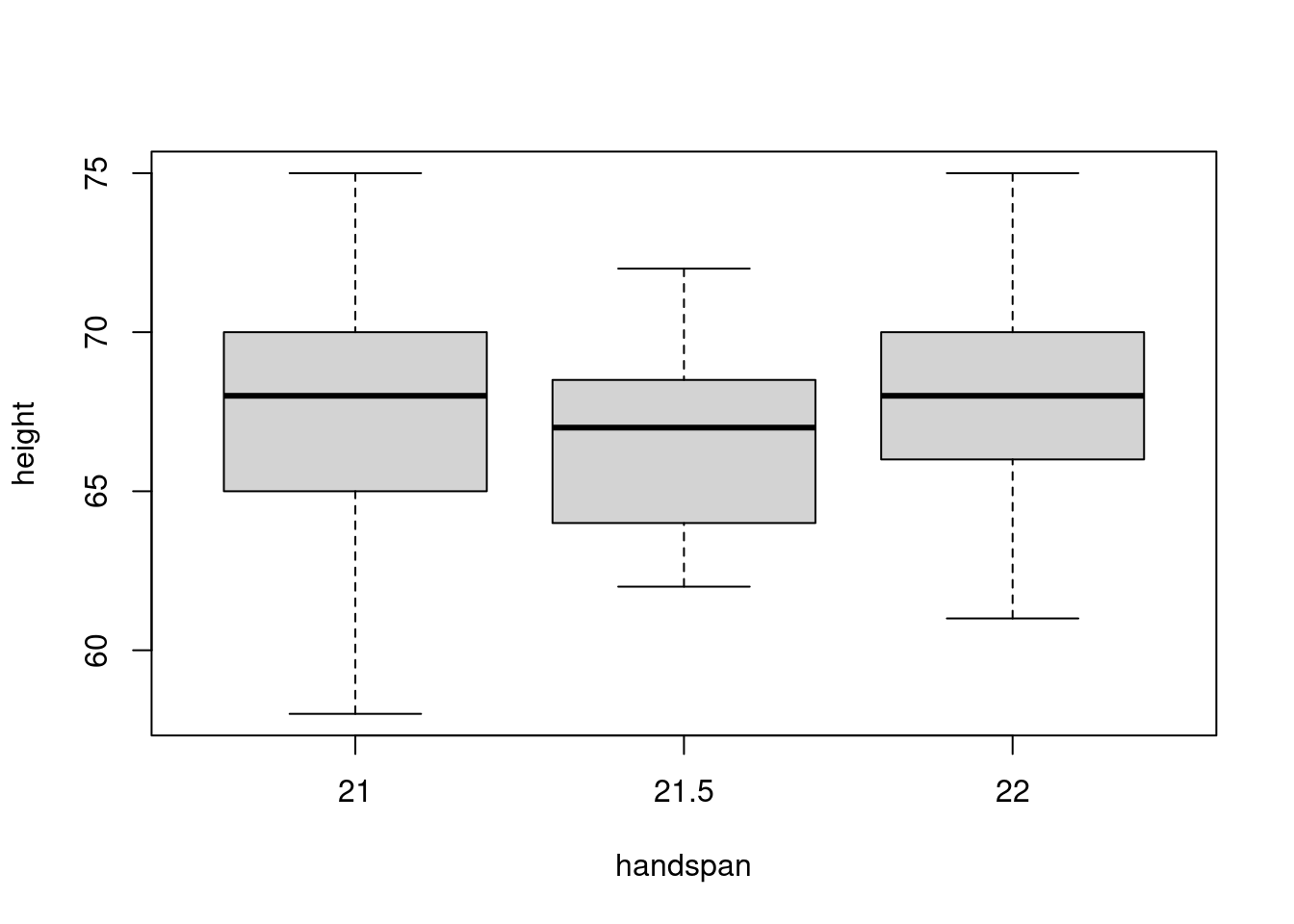

There’s a considerable amount of variation in peak for a given worth of handspan. Certainly, from this boxplot alone you may not even guess that there’s a robust constructive relationship between peak and handspan within the dataset as an entire! The “containers” within the determine, representing the center 50% of heights for a given handspan, overlap considerably. If we had been to randomly select one scholar with a handspan of 21 and one other with a handspan of 21.5, it’s fairly probably that the slope between them can be unfavourable. It’s true that college students with greater arms are taller on common. However the distinction in peak that we’d predict for 2 college students who differed by 0.5cm in handspan may be very small: 0.6 inches in keeping with the linear regression from the start of this put up. In distinction, the usual deviation of peak amongst college students with the median handspan is greater than 5 occasions as giant:

sd(subset(dat, handspan == 21.5)$peak)

## [1] 3.172248

The twenty fifth percentile of handspan is 20 whereas the seventy fifth percentile is 23. Evaluating the heights of scholars with these handspans somewhat than these near the median, offers a really completely different image:

boxplot(peak ~ handspan, dat, subset = handspan %in% c(20, 23))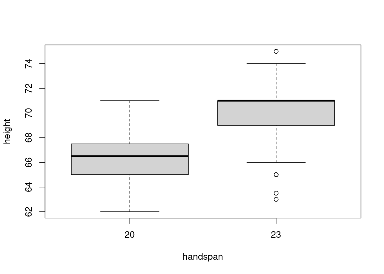

Now there’s a lot much less overlap within the distributions of peak. This accords with the predictions of the linear regression from above: for 2 college students whose handspan differs by 3cm, we might predict a distinction of three.8 inches in peak. This distinction is large enough to discern regardless of the variation in peak for college kids with the identical handspan. If we had been to decide on one scholar with a handspan of 20cm and one other with a handspan of 23cm, it’s pretty unlikely that the slope between these strains can be unfavourable.

So the place does this depart us? Above we noticed that forming a pair of scholars with the similar handspan doesn’t permit us to calculate a slope. Now we’ve seen that the slope for a pair of scholars with a really related handspan can provide a deceptive impression in regards to the total relationship. This seems to be the important thing to our puzzle from above. The unusual least squares slope estimate does equal a mean of the slopes for every pair of scholars, however this common offers extra weight to pairs with a bigger distinction in handspan. As I’ll derive in my subsequent put up:
[
widehat{beta}_{text{OLS}} = sum_{(i,j)in C_2^n} omega_{ij} left(frac{y_i – y_j}{x_i – x_j}right), quad
omega_{ij} equiv frac{(x_i – x_j)^2}{sum_{(i,j)in C_2^n} (x_i-x_j)^2}
]
The notation (C_2^n) is shorthand for the set ({(i,j)colon 1 leq i < j leq n}), in different phrases the set of all distinctive pairs ((i,j)) the place order doesn’t matter. The weights (omega_{ij}) are between zero and one and sum to at least one over all pairs. Pairs with (x_i = x_j) are given zero weight; pairs through which (x_i) is much from (x_j) are given extra weight than pairs the place these values are nearer. And also you don’t have to attend for my subsequent put up to see that it really works:

regression_pairs <- regression_pairs %>%
  mutate(x_dist = abs(x2 - x1),
         weight = x_dist^2 / sum(x_dist^2))

regression_pairs %>%
  filter(!is.infinite(slope) & !is.na(slope)) %>%
  summarize(sum(weight * slope)) %>%
  pull

## [1] 1.266961

coef(lm(peak ~ handspan, dat))[2]

## handspan 
## 1.266961

So there you could have it: in a easy linear regression, the OLS slope estimate is a weighted common of the slopes of the road segments between all pairs of observations. The weights are proportional to the squared Euclidean distance between (x)-coordinates. I’ll depart issues right here for at the moment, however there’s way more to say on this matter. Keep tuned for the subsequent installment!