Tips on how to create animated graphics for instance spatial spillover results

This publish reveals how you can create animated graphics that illustrate the spatial spillover results generated by a spatial autoregressive (SAR) mannequin. After studying this publish, you possibly can create an animated graph like the next.

This publish is organized as follows. First, I estimate the parameters of a SAR mannequin. Second, I present why a SAR mannequin can produce spatial spillover results. Lastly, I present how you can create an animated graph that illustrates the spatial spillover results.

A SAR mannequin

I need to analyze the murder fee in Texas counties as a operate of unemployment. I think that the murder fee in a single county impacts the murder fee in neighboring counties.

I need to reply two questions.

1. How can I arrange a mannequin that explicitly permits the murder fee in a single county to rely on the murder fee in neighboring counties?

2. Given my mannequin, if the unemployment fee in Dallas will increase to 10%, how would the murder fee change within the neighboring counties of Dallas ?

Match a SAR mannequin

An ordinary linear mannequin for the murder fee in county (i) (({bf hrate}_i)) as a operate of the unemployment fee in that county’s ({bf unemployment}_i) is

[begin{align} {bf hrate}_i = beta_0 + beta_1 {bf unemployment}_{i} + epsilon_i end{align} ]

A SAR mannequin permits ({bf hrate}_i) to rely on the murder fee in neighboring counties. I would like some new notation to jot down down a SAR mannequin. I let (W_{i,j}) be a constructive quantity if county (j) is a neighbor of county (i), zero if the (j) shouldn’t be a neighbor of (i), and 0 if (j=i), as a result of no county can border itself.

Given this notation, a SAR mannequin that enables the murder fee in county (i) to rely on the murder fee in neighboring counties might be written as

[ begin{align} {bf hrate}_i = gamma_1sum_{j=1}^N W_{i,j} {bf hrate}_{j} + beta_1 {bf unemployment}_{i} + beta_0 + epsilon_i end{align} ]

the place (W_{i,j}) defines the closeness between county (i) and county (j). The time period (sum_{j=1}^N W_{i,j} {bf hrate}_{j}) is a weighted sum of the murder charges in county (i)’s neighboring counties, and it specifies how the murder charges in neighboring counties have an effect on the murder fee in county (i).

Stacking the neighborhood info in (W_{i,j}) for every county (i) produces a matrix ({bf W}) that data the neighbor info for every county (i). The matrix ({bf W}) is called a spatial-weighting matrix.

The spatial-weighting matrix that we’re utilizing has a particular construction; every component is both a worth (c) or zero, the place (c) is larger than zero. The sort of spatial-weighting matrix is called a normalized contiguity matrix.

In Stata, we use spmatrix to create a spatial-weighting matrix, and we use spregress to suit a cross-sectional SAR mannequin.

I start by downloading some knowledge on the murder charges of U.S. counties from the Stata web site and making a subsample that makes use of solely knowledge on counties in Texas.

. /* Get knowledge for Texas counties' murder fee */
. copy http://www.stata-press.com/knowledge/r15/homicide1990.dta ., exchange

. use homicide1990
(S.Messner et al.(2000), U.S southern county murder charges in 1990)

. preserve if sname == "Texas"
(1,158 observations deleted)

. save texas, exchange
file texas.dta saved

Intuitively, a file that specifies the borders of all of the locations of curiosity is called a form file. texas.dta is linked to the Stata model of a form file that specifies the borders of all of the counties in Texas. I now obtain that dataset from the Stata web site and use spset to indicate that they’re linked.

. /* Get knowledge for Texas counties' murder fee */
. copy http://www.stata-press.com/knowledge/r15/homicide1990_shp.dta ., exchange

. spset
  Sp dataset texas.dta
                knowledge:  cross sectional
     spatial-unit id:  _ID
         coordinates:  _CX, _CY (planar)
    linked shapefile:  homicide1990_shp.dta

I now use spmatrix to create a normalized contiguity spatial-weighting matrix.

. /* Create a spatial contiguity matrix */
. spmatrix create contiguity W

Now that I’ve my knowledge and my spatial-weighting matrix, I can estimate the mannequin parameters.

. /* Estimate SAR mannequin parameters */
. spregress hrate unemployment, dvarlag(W) gs2sls
  (254 observations)
  (254 observations (locations) used)
  (weighting matrix defines 254 locations)

Spatial autoregressive mannequin                    Variety of obs     =        254
GS2SLS estimates                                Wald chi2(2)      =      14.23
                                                Prob > chi2       =     0.0008
                                                Pseudo R2         =     0.0424

------------------------------------------------------------------------------
       hrate |      Coef.   Std. Err.      z    P>|z|     [95% Conf. Interval]
-------------+----------------------------------------------------------------
hrate        |
unemployment |   .4584241    .152503     3.01   0.003     .1595237    .7573245
       _cons |   2.720913   1.653105     1.65   0.100    -.5191143    5.960939
-------------+----------------------------------------------------------------
W            |
       hrate |   .3414964   .1914865     1.78   0.075    -.0338103    .7168031
------------------------------------------------------------------------------
Wald check of spatial phrases:          chi2(1) = 3.18       Prob > chi2 = 0.0745

Spatial spillover

Now we’re able to reply the second query. Primarily based on our estimation outcomes from spregress, we are able to proceed in three steps.

1. Predict the murder fee utilizing authentic knowledge.

2. Change Dallas’s unemployment fee to 10% and predict the murder fee once more.

3. Compute the distinction between two predictions and map it.

. protect /* save knowledge briefly */

. /* Step 1: predict murder fee utilizing authentic knowledge */
. predict y0
(possibility rform assumed; reduced-form imply)

. /* Step 2: change Dallas unemployment fee to 10%, and predict once more*/
. exchange unemployment = 10 if cname == "Dallas"
(1 actual change made)

. predict y1
(possibility rform assumed; reduced-form imply)

. /* Step 3: Compute the prediction distinction and map it*/
. generate double y_diff = y1 - y0

. grmap y_diff, title("World spillover")

. restore /* return to authentic knowledge */

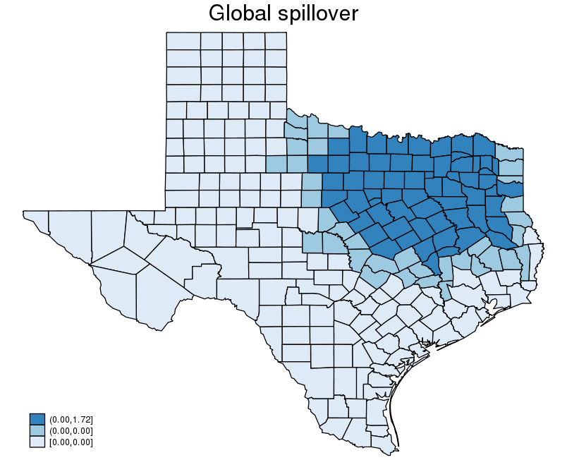
The above graph reveals {that a} change within the unemployment fee in Dallas adjustments the murder charges within the counties which might be close to to Dallas, along with the murder fee in Dallas. The change in Dallas spills over to the close by counties, and the impact is called a spillover impact.

SAR mannequin and spatial spillover

On this part, I present why a SAR mannequin generates a spillover impact. Within the course of, I present a formulation for this impact that I exploit to create the animated graph.

The matrix type for a SAR mannequin is

[begin{align} {bf y} &= lambda {bf W} {bf y} + {bf X}beta + epsilon end{align} ]

Fixing for ({bf y}) yields

[ begin{align} {bf y} &= ({bf I} – lambda {bf W})^{-1} {bf X}beta + epsilon
end{align} ]

The imply worth of ({bf y}) given a worth of ({bf X}) is called the the expectation of ({bf y}) conditional on ({bf X}). As a result of (epsilon) is unbiased of ({bf X}), the expectation of ({bf y}) conditional on ({bf X}) is

[begin{align} E({bf y}|{bf X}) &= ({bf I} – lambda {bf W})^{-1} {bf X}beta end{align} ]

Be aware that this conditional expectation specifies the imply for every county in Texas as a result of ({bf y}) is a vector.

We use this equation to outline the impact of going from one set of values for ({bf X}) to a different set. Within the case at hand, I let ({bf X_0}) comprise the covariate values within the noticed knowledge and let ({bf X_1}) comprise the identical values besides that the unemployment fee in Dallas has been set to 10%. With this notation, I see that going from ({bf X_0}) to ({bf X_1}) causes the imply murder charges for every county in Texas to vary by

[ begin{align} E({bf y}|{bf X_1}) – E({bf y}|{bf X_0}) &= ({bf I} – lambda {bf W})^{-1} {bf X_1} beta – ({bf I}- lambda {bf W})^{-1} {bf X_0} beta nonumber &=({bf I} – lambda {bf W})^{-1} Delta {bf X} beta tag{1} end{align} ]

[ begin{align} ({bf I} – lambda {bf W})^{-1} &= ({bf I} + lambda {bf W} + lambda^2 {bf W}^2 + lambda^3 {bf W}^3 + ldots) tag{2} end{align} ]

Plugging the formulation from (2) into the impact in (1) yields

[ begin{align} E({bf y}|{bf X_1}) – E({bf y}|{bf X_0}) &= ({bf I} – lambda {bf W})^{-1} Delta {bf X} beta nonumber &= ({bf I} + lambda {bf W} + lambda^2 {bf W}^2 + lambda^3 {bf W}^3 + ldots)Delta {bf X} beta nonumber &= Delta {bf X} beta + lambda {bf W} Delta {bf X}beta + lambda^2 {bf W}^2 Delta {bf X}beta + lambda^3 {bf W}^3 Delta {bf X} beta + ldots tag{3} end{align} ]

Every time period in (3) has some instinct, which is most simply introduced when it comes to my instance. The primary time period ((Delta {bf X}beta)) is the preliminary impact of the change, and it impacts solely the murder fee in Dallas. The second time period ((lambda {bf W} Delta {bf X}beta)) is the impact of the change on the end result in these locations which might be neighbors of Dallas. The third time period ((lambda^2 {bf W}^2 Delta {bf X}beta)) is the impact of the change on the end result in these locations which might be neighbors of neighbors of Dallas. The instinct continues within the sample for the remaining phrases.

Create animated graphs for spillover results

I now describe how I generate the animated graph. Every graph plots the change utilizing a subset of the phrases in (3). The primary graph plots the change computed from the primary time period solely. The second graph plots the change computed from the primary and second phrases solely. The third graph plots the change computed from the primary three phrases solely. And so forth.

The primary 4 steps of the code do the next.

1. It computes and plots (Delta {bf X}beta).

2. It computes and plots (Delta {bf X} beta + lambda {bf W} Delta {bf X}beta).

3. It compute and plots (Delta {bf X} beta + lambda {bf W} Delta {bf X}beta + lambda^2 {bf W}^2 Delta {bf X}beta).

4. It computes and plots (Delta {bf X} beta + lambda {bf W} Delta {bf X}beta + lambda^2 {bf W}^2 Delta {bf X}beta + lambda^3 {bf W}^3 Delta {bf X} beta).

Steps 5 by means of 20 carry out the analogous operations.

Lastly, mix graphs from step 1 to step 20, and create an animated graph.

Right here is the code that implements this course of.

  1 /* get estimate of spatial lag parameter lambda */
  2 native lambda = _b[W:hrate]
  3
  4 /* xb primarily based on authentic knowledge */
  5 predict xb0, xb
  6
  7 /* xb primarily based on modified knowledge */
  8 exchange unemployment = 10 if cname == "Dallas"
  9 predict xb1, xb
 10
 11 /* compute the end result change in step one */
 12 generate dy = xb1 - xb0
 13 format dy %9.2f
 14
 15 /* Initialize Wy, lamWy, */
 16 generate Wy = dy
 17 generate lamWy = dy
 18
 19 /* map the end result change in step 1 */
 20 grmap dy
 21 graph export dy_0.png, exchange
 22 native enter dy_0.png
 23
 24 /* compute the end result change from step 2 to 11 */
 25 forvalues p=1/20 {
 26         spgenerate tmp = W*Wy
 27         exchange lamWy = `lambda'^`p'*tmp
 28         exchange Wy = tmp
 29         exchange dy = dy + lamWy
 30         grmap dy
 31         graph export dy_`p'.png, exchange
 32         native enter `enter' dy_`p'.png
 33         drop tmp
 34 }
 35
 36 /* convert graphs right into a animated graph */
 37 shell convert -delay 150 -loop 0 `enter' glsp.gif
 38
 39 /* delete the generated pgn file */
 40 shell rm -fR *.png

This code makes use of the ereturn outcomes produced by spregress above and its corresponding predict command.

Line 2 places the estimate of (lambda) within the native macro lambda.

Strains 5, 7, 8, and 9 compute ({bf X}beta) for ({bf X_0}) and ({bf X_1}) and retailer them in xb0 and xb1, respectively.

Line 12 computes the primary time period ((Delta {bf X}beta)) and shops it in dy.

Strains 16 and 17 retailer the preliminary values for ({bf W}^{p} {bf y}) and (lambda^{p} {bf W}^{p} {bf y}), when (p=0).

Strains 20–22 produce the primary plot within the animated graph. The native macro enter will comprise all of the plots used to create the animated graph when the code finishes.

Strains 25–34 compute the phrases and create the plots for the remaining phrases. Line 26 makes use of spgenerate to compute ({bf W}^{p} {bf y}). Line 27–33 carry out operations analogous to these of dy.

In Line 37, I exploit a Linux device “convert” to mix the graphs to supply an animated graph. On Home windows, I can use software program equivalent to FFmpeg and Camtasia. For extra particulars, see Tips on how to create animated graphics utilizing Stata by Chuck Huber.

Line 40 deletes all of the pointless .png recordsdata.

Right here is the animated graph created by this code.

Achieved and undone

On this publish, I mentioned spillover results and why SAR fashions produce them within the context of an instance utilizing the counties in Texas. I additionally confirmed how the consequences might be computed as an gathered sum. I used the gathered sum to create an animated graph that illustrates how the consequences spill over within the counties in Texas.