

What are DSGE fashions?
Dynamic stochastic normal equilibrium (DSGE) fashions are utilized by macroeconomists to mannequin a number of time collection. A DSGE mannequin relies on financial principle. A principle could have equations for a way people or sectors within the financial system behave and the way the sectors work together. What emerges is a system of equations whose parameters could be linked again to the selections of financial actors. In lots of financial theories, people take actions based mostly partly on the values they count on variables to absorb the long run, not simply on the values these variables take within the present interval. The power of DSGE fashions is that they incorporate these expectations explicitly, in contrast to different fashions of a number of time collection.
DSGE fashions are sometimes used within the evaluation of shocks or counterfactuals. A researcher would possibly topic the mannequin financial system to an sudden change in coverage or the surroundings and see how variables reply. For instance, what’s the impact of an sudden rise in rates of interest on output? Or a researcher would possibly examine the responses of financial variables with totally different coverage regimes. For instance, a mannequin may be used to match outcomes beneath a high-tax versus a low-tax regime. A researcher would discover the habits of the mannequin beneath totally different settings for tax charge parameters, holding different parameters fixed.
On this submit, I present you easy methods to estimate the parameters of a DSGE mannequin, easy methods to create and interpret an impulse response, and easy methods to examine the impulse response estimated from the information with an impulse response generated by a counterfactual coverage regime.
Estimate mannequin parameters
I’ve month-to-month information on the expansion charge of business manufacturing and rates of interest. I’ll use these information to estimate the parameters of a small DSGE mannequin. My mannequin has simply two brokers: corporations that produce output (ip) and a central financial institution that units rates of interest (r). In my mannequin, industrial manufacturing progress depends upon the anticipated rate of interest one interval sooner or later and on different exogenous elements. In flip, the rate of interest depends upon contemporaneous industrial manufacturing progress and on different latent elements. I name the latent elements affecting manufacturing e and the latent elements affecting rates of interest m.
The latent elements are often called “state variables” within the jargon. We will impose a shock to state variables and hint out how that shock impacts the system. I specify the evolution of m as an AR(1) course of. To provide the mannequin some further dynamics, I specify the evolution of e as an AR(2) course of. My full mannequin is
start{align}label{eq:fullmodel}
ip_t &= alpha E(r_{t+1}) + e_t tag{1}
r_t &= beta ip_t + m_t tag{2}
m_{t+1} &= rho m_t + v_{t+1} tag{3}
e_{t+1} &= theta_{1} e_t + theta_{2} e_{t-1} + u_{t+1} tag{4}
finish{align}
Earlier than I talk about these equations in additional element, let’s estimate the parameters with dsge.
. dsge    (ip   = {alpha}*E(F.r) + e)
>         (r    = {beta}*ip + m )
>         (F.m  = {rho}*m, state)
>         (F.e  = {theta1}*e + {theta2}*Le, state)
>         (F.Le = e, state noshock), nolog

DSGE mannequin

Pattern: 1954m7 - 2006m12                        Variety of obs     =        630
Log probability = -2284.7062
------------------------------------------------------------------------------
             |                 OIM
             |      Coef.   Std. Err.      z    P>|z|     [95% Conf. Interval]
-------------+----------------------------------------------------------------
/structural  |
       alpha |  -.6287781   .2148459    -2.93   0.003    -1.049868   -.2076878
        beta |   .0239873   .0056561     4.24   0.000     .0129016     .035073
         rho |   .9870175   .0060728   162.53   0.000      .975115      .99892
      theta1 |    1.13085   .0364878    30.99   0.000     1.059335    1.202365
      theta2 |  -.3731307   .0364835   -10.23   0.000     -.444637   -.3016244
-------------+----------------------------------------------------------------
      sd(e.m)|   .5464261   .0155047                      .5160374    .5768148
      sd(e.e)|   4.079367   .1176248                      3.848827    4.309908
------------------------------------------------------------------------------
The primary equation is the manufacturing equation. We write (1) in Stata as (ip = {alpha}*E(F.r) + e). This equation specifies industrial manufacturing progress as a operate of anticipated future rates of interest. This rate of interest seems on this equation inside an E() operator; E(F.r) represents the anticipated worth of the rate of interest one interval forward. Consider alpha as a parameter set by corporations and brought as given by policymakers. The estimated worth of alpha is damaging, implying that industrial manufacturing progress falls when corporations count on to face a interval of upper rates of interest.
The second equation is the rate of interest equation. We write (2) in Stata as (r = {beta}*ip + m). Consider beta as a parameter set by policymakers; it measures how strongly policymakers react to adjustments in manufacturing. We see that the estimate of beta is optimistic. Policymakers have a tendency to extend rates of interest when manufacturing is excessive and minimize rates of interest when manufacturing is low. Nevertheless, the estimated response coefficient is pretty small. We’ll consider the coefficient on ip as representing systematic coverage (how policymakers reply to industrial manufacturing immediately) and consider the state variable m as representing discretionary coverage (or different elements that have an effect on rates of interest in addition to coverage).
The third equation is a first-order autoregressive equation for m, the variable capturing discretionary coverage that impacts rates of interest. We write (3) in Stata as (F.m = {rho}*m, state). State variables are predetermined, so the timing conference in dsge is that state equations are specified when it comes to the worth of the state variable one interval forward (F.m). State equations are additionally marked off with the state choice. The error (v_{t+1}) is included by default. The estimated autoregressive parameter rho is optimistic and captures the persistence of the rate of interest.
The mannequin has 4 equations, however the dsge command contains 5 equations. Equation (4) specifies an AR(2) course of for exogenous elements affecting industrial manufacturing progress. To specify this equation to dsge, I want to interrupt it up into two items, and people two items develop into the final two equations within the mannequin. For full particulars, see the footnote on the finish of this submit. The parameters in these equations theta1 and theta2 seize persistence in industrial manufacturing progress.
Discover a shock to the mannequin: Impulse responses
We subsequent add shocks into the mannequin and hint out their results on industrial manufacturing. To do that, we have to set an impulse–response operate (IRF) file and retailer the estimates in it. The irf set command creates a file, dsge_irf.irf, to carry our IRFs. The irf create estimated command creates a set of impulse responses utilizing the present dsge estimates. irf create creates a full set of all responses to all doable impulses. In our mannequin, which means each state variables e and m are shocked, and the response is recorded for each ip and r. Lastly, we’ll use the irf graph irf command to decide on which responses to plot and which impulses are driving these responses. We solely plot the response of ip for every of the impulses e and m.
. irf set dta/dsge_irf, exchange
(file dta/dsge_irf.irf created)
(file dta/dsge_irf.irf now energetic)

. irf create estimated, step(24)
(file dta/dsge_irf.irf up to date)

. irf graph irf, impulse(e m) response(ip) byopts(yrescale)
> xlabel(0(3)24) yline(0)
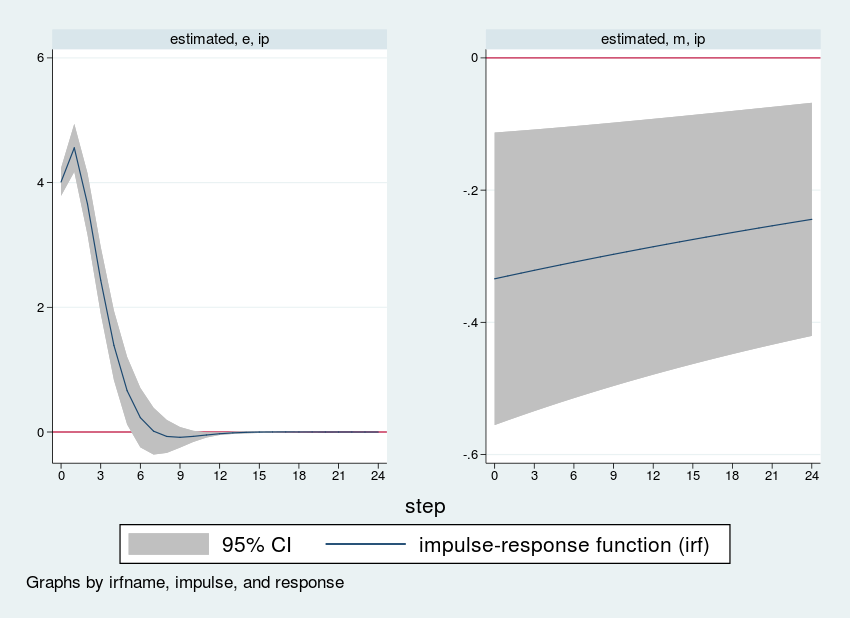
Every panel exhibits the response of business manufacturing to 1 shock. As a result of our information are measured in progress charges, the vertical axis can be measured in progress charges. Therefore, a price of “4” within the left-hand panel implies that after a one standard-deviation shock, industrial manufacturing grows 4 proportion factors sooner than it in any other case would. The horizontal axis is time; as a result of we used month-to-month information, it’s time in months, and 12 steps represents 1 12 months.
The left-hand panel exhibits the response of business manufacturing to an increase in e, the latent issue affecting manufacturing. Industrial manufacturing rises, peaking one interval after the shock earlier than settling again all the way down to long-run equilibrium. The impact of the shock wears off rapidly; industrial manufacturing returns to long-run equilibrium inside 12 durations (1 12 months of month-to-month observations).
The fitting-hand panel exhibits the response of business manufacturing to an increase in m, which has a pure interpretation as an sudden hike in rates of interest. The scale of a shock is one customary deviation, which from the dsge estimates desk above is an sudden rise in rates of interest of about 0.546, or about one-half of 1 proportion level. In response, we see within the graph that industrial manufacturing progress falls by about one-third of 1 proportion level and stays low for over 24 durations. All variables in a DSGE mannequin are stationary, so in the long term, the impact of a shock dies off, and the variables return to their long-run imply of zero.
Discover systematic coverage: A change in regime
Subsequent, we ponder a shift in coverage regime. Suppose the policymaker receives directions to easy out fluctuations in industrial manufacturing ensuing from shocks to e. By way of the mannequin, this directive could be represented by a regime shift from the comparatively low response coefficient beta seen within the information to the next response coefficient.
dsge with the from() and clear up choices lets you hint out an impulse response from any arbitrary parameter set. We’ll make the most of this function now. First, we retailer the estimated parameter vector in a Stata matrix:
. matrix b2 = e(b)
Subsequent, we exchange the coefficient beta with a bigger response coefficient. For illustrative functions, I exploit a response coefficient of 0.8 as a substitute of 0.02. The outdated and new parameter vectors are
. matrix b2[1,2] = 0.8

. matlist e(b)

             | /struct~l                                             | /
             |     alpha       beta        rho     theta1     theta2 |   sd(e.m)
-------------+-------------------------------------------------------+-----------
          y1 | -.6287781   .0239873   .9870175    1.13085  -.3731307 |  .5464261

             | /
             |   sd(e.e)
-------------+-----------
          y1 |  4.079367

. matlist b2

             | /struct~l                                             | /
             |     alpha       beta        rho     theta1     theta2 |   sd(e.m)
-------------+-------------------------------------------------------+-----------
          y1 | -.6287781         .8   .9870175    1.13085  -.3731307 |  .5464261

             | /
             |   sd(e.e)
-------------+-----------
          y1 |  4.079367
As anticipated, they’re similar aside from the beta entry. Subsequent, we rerun dsge on the new parameter vector with from() and clear up.
. dsge (ip = {alpha}*E(F.r) + e)
>         (r = {beta}*ip + m )
>         (F.m = {rho}*m, state)
>         (F.e = {theta1}*e + {theta2}*Le, state)
>         (F.Le = e, state noshock)
>         , from(b2) clear up

DSGE mannequin

Pattern: 1954m7 - 2006m12                        Variety of obs     =        630
Log probability = -15344.268
------------------------------------------------------------------------------
             |                 OIM
             |      Coef.   Std. Err.      z    P>|z|     [95% Conf. Interval]
-------------+----------------------------------------------------------------
/structural  |
       alpha |  -.6287781          .        .       .            .           .
        beta |         .8          .        .       .            .           .
         rho |   .9870175          .        .       .            .           .
      theta1 |    1.13085          .        .       .            .           .
      theta2 |  -.3731307          .        .       .            .           .
-------------+----------------------------------------------------------------
      sd(e.m)|   .5464261          .                             .           .
      sd(e.e)|   4.079367          .                             .           .
------------------------------------------------------------------------------
Word: Mannequin solved at specified parameters.
We use these new parameter values to create a brand new set of IRFs that we name counterfactual.
. irf create counterfactual, step(24)
(file dta/dsge_irf.irf up to date)
Lastly, we plot the responses beneath the estimated and counterfactual parameter vectors with irf ograph:
. irf ograph (estimated e ip irf) (counterfactual e ip irf),
> xlabel(0(3)24) yline(0)
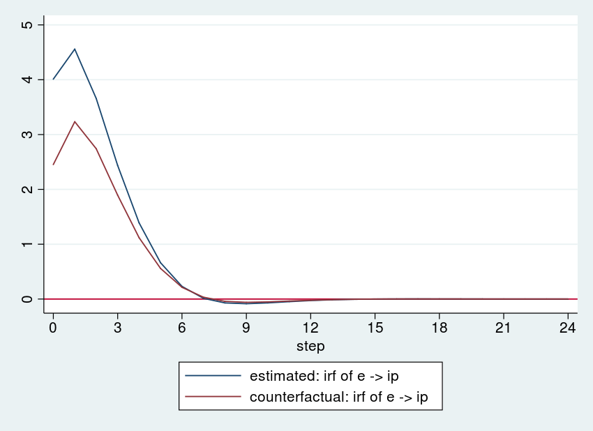
The extra aggressive coverage has dampened the response of business manufacturing to the e shock. The policymaker may experiment with different values of beta till she or he discovered a price that dampened the response of business manufacturing by the specified quantity.
Appendix
Knowledge
I used information on the expansion charge of business manufacturing and on the Federal funds rate of interest. Each of those collection can be found month-to-month on the St. Louis Federal Reserve database, FRED. The Stata command import fred imports information from FRED. The codes are INDPRO for industrial manufacturing and FEDFUNDS for the Federal funds charge.
I generate the variable ip because the annualized quarterly progress charge of business manufacturing and use a pattern from 1954 to 2006.
. import fred INDPRO FEDFUNDS
. generate datem = mofd(daten)
. tsset datem, month-to-month
. generate ip = 400*ln(INDPRO / L3.INDPRO)
. label variable ip "Progress charge of business manufacturing"
. rename FEDFUNDS r
. label variable r "Federal funds charge"
. maintain if yofd(daten) <= 2006
Specifying state equations with lengthy lags
See additionally [DSGE] intro 4c.
Discover that state variables are written in a state-space kind when it comes to their one-period-ahead worth. For an AR(1) course of, that is straightforward. The equation
start{align*}
m_{t+1} &= rho m_t + v_{t+1}
finish{align*}
turns into the next in Stata:
. dsge ... (F.m = {rho}*m, state) ...
However for an AR(2) course of, the regulation of movement for the state variable is
start{align*}
e_{t+1} &= theta_{1} e_t + theta_{2} e_{t-1} + u_{t+1}
finish{align*}
which we break up into two equations:
start{align*}
start{pmatrix} e_{t+1} e_t finish{pmatrix}
=
start{pmatrix}
theta_{1} & theta_{2}
1 & 0
finish{pmatrix}
start{pmatrix}
e_t e_{t-1}
finish{pmatrix}
+
start{pmatrix}
u_t 0
finish{pmatrix}
finish{align*}
These two equations develop into, in Stata,
. dsge ... (F.e = {theta1}*e + {theta2}*Le, state) (F.Le = e, state noshock) ...
the place the noshock choice within the final equation specifies that it’s actual.
See additionally [TS] sspace instance 5, the place the same trick is used.