

Why is the lasso fascinating?
The least absolute shrinkage and choice operator (lasso) estimates mannequin coefficients and these estimates can be utilized to pick out which covariates ought to be included in a mannequin. The lasso is used for final result prediction and for inference about causal parameters. On this publish, we offer an introduction to the lasso and talk about utilizing the lasso for prediction. Within the subsequent publish, we talk about utilizing the lasso for inference about causal parameters.
The lasso is most helpful when a couple of out of many potential covariates have an effect on the result and you will need to embody solely the covariates which have an have an effect on. “Few” and “many” are outlined relative to the pattern dimension. Within the instance mentioned under, we observe the newest health-inspection scores for 600 eating places, and we’ve 100 covariates that might doubtlessly have an effect on every one’s rating. We’ve too many potential covariates as a result of we can not reliably estimate 100 coefficients from 600 observations. We imagine that solely about 10 of the covariates are vital, and we really feel that 10 covariates are “a couple of” relative to 600 observations.
On condition that just a few of the various covariates have an effect on the result, the issue is now that we don’t know which covariates are vital and which aren’t. The lasso produces estimates of the coefficients and solves this covariate-selection drawback.
There are technical phrases for our instance state of affairs. A mannequin with extra covariates than whose coefficients you possibly can reliably estimate from the obtainable pattern dimension is called a high-dimensional mannequin. The idea that the variety of coefficients which can be nonzero within the true mannequin is small relative to the pattern dimension is called a sparsity assumption. Extra realistically, the approximate sparsity assumption requires that the variety of nonzero coefficients within the mannequin that greatest approximates the actual world be small relative to the pattern dimension.
In these technical phrases, the lasso is most helpful when estimating the coefficients in a high-dimensional, roughly sparse, mannequin.
Excessive-dimensional fashions are practically ubiquitous in prediction issues and fashions that use versatile purposeful kinds. In lots of circumstances, the various potential covariates are created from polynomials, splines, or different features of the unique covariates. In different circumstances, the various potential covariates come from administrative information, social media, or different sources that naturally produce enormous numbers of potential covariates.
Predicting restaurant inspection scores
We use a sequence of examples to make our dialogue of the lasso extra accessible. These examples use some simulated information from the next drawback. A well being inspector in a small U.S. metropolis desires to make use of social-media evaluations to foretell the health-inspection scores of eating places. The inspector plans so as to add shock inspections to the eating places with the lowest-predicted well being scores, utilizing our predictions.
hsafety2.dta has 1 commentary for every of 600 eating places, and the rating from the newest inspection is in rating. The share of a restaurant’s social-media evaluations that comprise a phrase like “soiled” might predict the inspection rating. We recognized 50 phrases, 30 phrase pairs, and 20 phrases whose incidence percentages in evaluations written within the three months previous to an inspection might predict the inspection rating. The incidence percentages of the 50 phrases are in word1 – word50. The incidence percentages of 30-word pairs are in wpair1 – wpair30. The incidence percentages of the 20 phrases are in phrase1 – phrase20.
Researchers broadly use the next steps to search out the perfect predictor.
- Divide the pattern into coaching and validation subsamples.
- Use the coaching information to estimate the mannequin parameters of every of the competing estimators.
- Use the validation information to estimate the out-of-sample imply squared error (MSE) of the predictions produced by every competing estimator.
- One of the best predictor is the estimator that produces the smallest out-of-sample MSE.
The unusual least-squares (OLS) estimator is ceaselessly included as a benchmark estimator when it’s possible. We start the method with splitting the pattern and computing the OLS estimates.
Within the output under, we learn the information into reminiscence and use splitsample with the choice break up(.75 .25) to generate the variable pattern, which is 1 for a 75% of the pattern and a couple of for the remaining 25% of the pattern. The project of every commentary in pattern to 1 or 2 is random, however the rseed possibility makes the random project reproducible.
. use hsafety2

. splitsample , generate(pattern) break up(.75 .25) rseed(12345)

. label outline slabel 1 "Coaching" 2 "Validation"

. label values pattern slabel

. tabulate pattern

     pattern |      Freq.     P.c        Cum.
------------+-----------------------------------
   Coaching |        450       75.00       75.00
 Validation |        150       25.00      100.00
------------+-----------------------------------
      Complete |        600      100.00
The one-way tabulation of pattern produced by tabulate verifies that pattern incorporates the requested 75%–25% division.
Subsequent, we compute the OLS estimates utilizing the information within the coaching pattern and retailer the leads to reminiscence as ols.
. quietly regress rating word1-word50 wpair1-wpair30 phrase1-phrase20
>         if pattern==1

. estimates retailer ols
Now, we use lassogof with possibility over(pattern) to compute the in-sample (Coaching) and out-of-sample (Validation) estimates of the MSE.
. lassogof ols, over(pattern)

Penalized coefficients
-------------------------------------------------------------
Title             pattern |         MSE    R-squared        Obs
------------------------+------------------------------------
ols                     |
               Coaching |    24.43515       0.5430        450
             Validation |    35.53149       0.2997        150
-------------------------------------------------------------
As anticipated, the estimated MSE is way smaller within the Coaching subsample than within the Validation pattern. The out-of-sample estimate of the MSE is the extra dependable estimator for the prediction error; see, for instance, chapters 1, 2, and three in Hastie, Tibshirani, and Friedman (2009).
On this part, we introduce the lasso and evaluate its estimated out-of-sample MSE to the one produced by OLS.
What’s a lasso?
The lasso is an estimator of the coefficients in a mannequin. What makes the lasso particular is that a few of the coefficient estimates are precisely zero, whereas others should not. The lasso selects covariates by excluding the covariates whose estimated coefficients are zero and by together with the covariates whose estimates should not zero. There are not any commonplace errors for the lasso estimates. The lasso’s skill to work as a covariate-selection technique makes it a nonstandard estimator and prevents the estimation of normal errrors. On this publish, we talk about how one can use the lasso for inferential questions.
Tibshirani (1996) derived the lasso, and Hastie, Tibshirani, and Wainwright (2015) present a textbook introduction.
The rest of this part supplies some particulars in regards to the mechanics of how the lasso produces its coefficient estimates. There are totally different variations of the lasso for linear and nonlinear fashions. Variations of the lasso for linear fashions, logistic fashions, and Poisson fashions can be found in Stata 16. We talk about solely the lasso for the linear mannequin, however the factors we make generalize to the lasso for nonlinear fashions.
Like many estimators, the lasso for linear fashions solves an optimization drawback. Particularly, the linear lasso level estimates (widehat{boldsymbol{beta}}) are given by
$$
widehat{boldsymbol{beta}} = argmin_{boldsymbol{beta}}
left{
frac{1}{2n} sum_{i=1}^nleft(y_i – {bf x}_iboldsymbol{beta}’proper)^2
+lambdasum_{j=1}^pomega_jvertbeta_jvert
proper}
$$
the place
- (lambda>0) is the lasso penalty parameter,
- (y) is the result variable,
- ({bf x}) incorporates the (p) potential covariates,
- (boldsymbol{beta}) is the vector of coefficients on ({bf x}),
- (beta_j) is the (j)th component of (boldsymbol{beta}),
- the (omega_j) are parameter-level weights often called penalty loadings, and
- (n) is the pattern dimension.
There are two phrases on this optimization drawback, the least-squares match measure
$$frac{1}{2n} sum_{i=1}^nleft(y_i – {bf x}_iboldsymbol{beta}’proper)^2$$
and the penalty time period
$$lambdasum_{j=1}^pomega_jvertboldsymbol{beta}_jvert$$
The parameters (lambda) and the (omega_j) are referred to as “tuning” parameters. They specify the burden utilized to the penalty time period. When (lambda=0), the linear lasso reduces to the OLS estimator. As (lambda) will increase, the magnitude of all of the estimated coefficients is “shrunk” towards zero. This skrinkage happens as a result of the price of every nonzero (widehat{beta}_j) will increase with the penalty time period that will increase as (lambda) will increase.
The penalty time period consists of absolutely the worth of every (beta_j). Absolutely the worth perform has a kink, generally referred to as a verify, at zero. The kink within the contribution of every coefficient to the penalty time period causes a few of the estimated coefficients to be precisely zero on the optimum resolution. See part 2.2 of Hastie, Tibshirani, and Wainwright (2015) for extra particulars.
There’s a worth (lambda_{rm max}) for which all of the estimated coefficients are precisely zero. As (lambda) decreases from (lambda_{rm max}), the variety of nonzero coefficient estimates will increase. For (lambdain(0,lambda_{rm max})), a few of the estimated coefficients are precisely zero and a few of them should not zero. If you use the lasso for covariate choice, covariates with estimated coefficients of zero are excluded, and covariates with estimated coefficients that aren’t zero are included.
That the variety of potential covariates (p) may be larger than the pattern dimension (n) is a a lot mentioned benefit of the lasso. It is very important keep in mind that the approximate sparsity assumption requires that the variety of covariates that belong within the mannequin ((s)) should be small relative to (n).
Choosing the lasso tuning parameters
The tuning parameters should be chosen earlier than utilizing the lasso for prediction or mannequin choice. Probably the most frequent strategies used to pick out the tuning parameters are cross-validation (CV), the adaptive lasso, and plug-in strategies. As well as, (lambda) is usually set by hand in a sensitivity evaluation.
CV finds the (lambda) that minimizes the out-of-sample MSE of the predictions. The mechanics of CV mimic the method utilizing break up samples to search out the perfect out-of-sample predictor. The small print are introduced in an appendix.
CV is the default technique of choosing the tuning parameters within the lasso command. Within the output under, we use lasso to estimate the coefficients within the mannequin for rating, utilizing the coaching pattern. We specified the choice rseed() to make our CV outcomes reproducible.
. lasso linear rating word1-word50 wpair1-wpair30 phrase1-phrase20
>         if pattern==1, nolog rseed(12345)

Lasso linear mannequin                          No. of obs        =        450
                                            No. of covariates =        100
Choice: Cross-validation                 No. of CV folds   =         10

--------------------------------------------------------------------------
         |                                No. of      Out-of-      CV imply
         |                               nonzero       pattern   prediction
      ID |     Description      lambda     coef.    R-squared        error
---------+----------------------------------------------------------------
       1 |    first lambda    3.271123         0       0.0022       53.589
      25 |   lambda earlier than    .3507518        22       0.3916     32.53111
    * 26 | chosen lambda     .319592        25       0.3917     32.52679
      27 |    lambda after    .2912003        26       0.3914     32.53946
      30 |     final lambda    .2202824        30       0.3794     33.18254
--------------------------------------------------------------------------
* lambda chosen by cross-validation.

. estimates retailer cv
We specified the choice nolog to supress the CV log over the candidate values of (lambda). The output reveals that CV chosen a (lambda) for which 25 of the 100 covariates have nonzero coefficients. We used estimates retailer to retailer these outcomes beneath the identify cv in reminiscence.
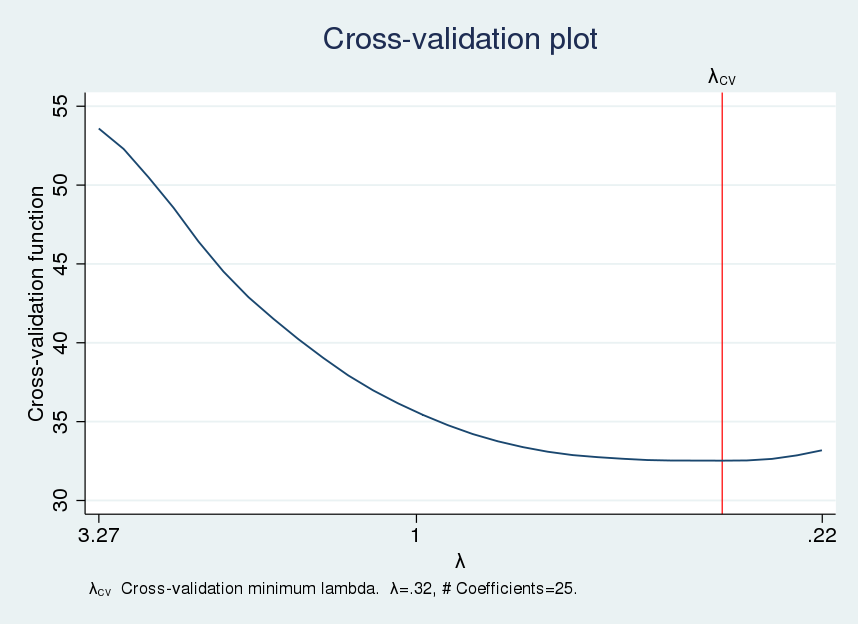
We use cvplot to plot the CV perform.
. cvplot, minmax
The CV perform seems considerably flat close to the optimum (lambda), which means that close by values of (lambda) would produce comparable out-of-sample MSEs.
The variety of included covariates can fluctuate considerably over the flat a part of the CV perform. We will examine the variation within the variety of chosen covariates utilizing a desk referred to as a lasso knot desk. Within the jargon of lasso, a knot is a price of (lambda) for which a covariate is added or subtracted to the set of covariates with nonzero values. We use lassoknots to show the desk of knots.
. lassoknots

-------------------------------------------------------------------------------------
       |              No. of   CV imply |
       |             nonzero     pred. |        Variables (A)dded, (R)emoved,
    ID |   lambda      coef.     error |             or left (U)nchanged
-------+-------------------------------+---------------------------------------------
     2 | 2.980526          2   52.2861 | A phrase3   phrase4
     3 | 2.715744          3  50.48463 | A phrase5
     4 | 2.474485          4  48.55981 | A word3
     6 | 2.054361          5  44.51782 | A phrase6
     9 | 1.554049          6  40.23385 | A wpair3
    10 | 1.415991          8  39.04494 | A wpair2    phrase2
    12 | 1.175581          9    36.983 | A word2
    14 | .9759878         10  35.42697 | A word31
    16 | .8102822         11   34.2115 | A word19
    17 |  .738299         12  33.75501 | A word4
    21 | .5088809         14  32.74808 | A word14    phrase7
    22 | .4636733         17  32.64679 | A word32    wpair19   wpair26
    23 | .4224818         19  32.56572 | A wpair15   wpair25
    24 | .3849497         22  32.53301 | A wpair24   phrase13  phrase14
  * 26 |  .319592         25  32.52679 | A word25    word30    phrase8
    27 | .2912003         26  32.53946 | A wpair11
    29 | .2417596         27  32.86193 | A wpair17
    30 | .2202824         30  33.18254 | A word23    word38    wpair4
-------------------------------------------------------------------------------------
* lambda chosen by cross-validation.
The CV perform is minimized on the (lambda) with ID=26, and the lasso consists of 25 covariates at this (lambda) worth. The flat a part of the CV perform consists of the (lambda) values with ID (in{21,22,23,24,26,27}). Solely 14 covariates are included by the lasso utilizing the (lambda) at ID=21. We’ll discover this commentary utilizing sensitivity evaluation under.
CV tends to incorporate further covariates whose coefficients are zero within the mannequin that greatest approximates the method that generated the information. This could have an effect on the prediction efficiency of the CV-based lasso, and it may possibly have an effect on the efficiency of inferential strategies that use a CV-based lasso for mannequin choice. The adaptive lasso is a multistep model of CV. It was designed to exclude a few of these further covariates.
Step one of the adaptive lasso is CV. The second step does CV among the many covariates chosen in step one. On this second step, the penalty loadings are (omega_j=1/| widehat{boldsymbol{beta}}_j|), the place (widehat{boldsymbol{beta}}_j) are the penalized estimates from step one. Covariates with smaller-magnitude coefficients usually tend to be excluded within the second step. See Zou (2006) and Bühlmann and Van de Geer (2011) for extra in regards to the adaptive lasso and the tendency of the CV-based lasso to overselect. Additionally see Chetverikov, Liao, and Chernozhukov (2019) for formal outcomes for the CV lasso and outcomes that might clarify this overselection tendency.
We specify the choice choice(adaptive) under to trigger lasso to make use of the adaptive lasso as an alternative of CV to pick out the tuning parameters. We used estimates retailer to retailer the outcomes beneath the identify adaptive.
. lasso linear rating word1-word50 wpair1-wpair30 phrase1-phrase20
>         if pattern==1, nolog rseed(12345) choice(adaptive)

Lasso linear mannequin                         No. of obs         =        450
                                           No. of covariates  =        100
Choice: Adaptive                        No. of lasso steps =          2

Last adaptive step outcomes
--------------------------------------------------------------------------
         |                                No. of      Out-of-      CV imply
         |                               nonzero       pattern   prediction
      ID |     Description      lambda     coef.    R-squared        error
---------+----------------------------------------------------------------
      31 |    first lambda    124.1879         0       0.0037     53.66569
      77 |   lambda earlier than    1.719861        12       0.4238     30.81155
    * 78 | chosen lambda    1.567073        12       0.4239      30.8054
      79 |    lambda after    1.427859        14       0.4237     30.81533
     128 |     final lambda    .0149585        22       0.4102     31.53511
--------------------------------------------------------------------------
* lambda chosen by cross-validation in remaining adaptive step.

. estimates retailer adaptive
We see that the adaptive lasso included 12 as an alternative of 25 covariates.
Plug-in strategies are typically much more parsimonious than the adaptive lasso. Plug-in strategies discover the worth of the (lambda) that’s giant sufficient to dominate the estimation noise. The plug-in technique chooses (omega_j) to normalize the scores of the (unpenalized) match measure for every parameter. Given the normalized scores, it chooses a price for (lambda) that’s larger than the most important normalized rating with a likelihood that’s near 1.
The plug-in-based lasso is way sooner than the CV-based lasso and the adaptive lasso. In follow, the plug-in-based lasso tends to incorporate the vital covariates and it’s actually good at not together with covariates that don’t belong within the mannequin that greatest approximates the information. The plug-in-based lasso has a threat of lacking some covariates with giant coefficients and discovering just some covariates with small coefficients. See Belloni, Chernozhukov, and Wei (2016) and Belloni, et al. (2012) for particulars and formal outcomes.
We specify the choice choice(plugin) under to trigger lasso to make use of the plug-in technique to pick out the tuning parameters. We used estimates retailer to retailer the outcomes beneath the identify plugin.
. lasso linear rating word1-word50 wpair1-wpair30 phrase1-phrase20
>         if pattern==1, choice(plugin)

Computing plugin lambda ...
Iteration 1:     lambda = .1954567   no. of nonzero coef. =       8
Iteration 2:     lambda = .1954567   no. of nonzero coef. =       9
Iteration 3:     lambda = .1954567   no. of nonzero coef. =       9

Lasso linear mannequin                          No. of obs        =        450
                                            No. of covariates =        100
Choice: Plugin heteroskedastic

--------------------------------------------------------------------------
         |                                No. of
         |                               nonzero    In-sample
      ID |     Description      lambda     coef.    R-squared          BIC
---------+----------------------------------------------------------------
     * 1 | chosen lambda    .1954567         9       0.3524     2933.203
--------------------------------------------------------------------------
* lambda chosen by plugin system assuming heteroskedastic.

. estimates retailer plugin
The plug-in-based lasso included 9 of the 100 covariates, which is much fewer than included by the CV-based lasso or the adaptive lasso.
Evaluating the predictors
We now have 4 totally different predictors for rating: OLS, CV-based lasso, adaptive lasso, and plug-in-based lasso. The three lasso strategies might predict rating utilizing the penalized coefficients estimated by lasso, or they may predict rating utilizing the unpenalized coefficients estimated by OLS, together with solely the covariates chosen by lasso. The predictions that use the penalized lasso estimates are often called the lasso predictions and the predictions that use the unpenalized coefficients are often called the postselection predictions, or the postlasso predictions.
For linear fashions, Belloni and Chernozhukov (2013) current circumstances through which the postselection predictions carry out no less than in addition to the lasso predictions. Heuristically, one expects the lasso predictions from a CV-based lasso to carry out higher than the postselection predictions as a result of CV chooses (lambda) to make the perfect lasso predictions. Analogously, one expects the postselection predictions for the plug-in-based lasso to carry out higher than the lasso predictions as a result of the plug-in tends to pick out a set of covariates shut to those who greatest approximate the method that generated the information.
In follow, we estimate the out-of-sample MSE of the predictions for all estimators utilizing each the lasso predictions and the postselection predictions. We choose the one which produces the bottom out-of-sample MSE of the predictions.
Within the output under, we use lassogof to check the out-of-sample prediction efficiency of OLS and the lasso predictions from the three lasso strategies.
. lassogof ols cv adaptive plugin if pattern==2

Penalized coefficients
-------------------------------------------------
       Title |         MSE    R-squared        Obs
------------+------------------------------------
        ols |    35.53149       0.2997        150
         cv |    27.83779       0.4513        150
   adaptive |    27.83465       0.4514        150
     plugin |    32.29911       0.3634        150
-------------------------------------------------
For these information, the lasso predictions utilizing the adaptive lasso carried out a bit of bit higher than the lasso predictions from the CV-based lasso.
Within the output under, we evaluate the out-of-sample prediction efficiency of OLS and the lasso predictions from the three lasso strategies utilizing the postselection coefficient estimates.
. lassogof ols cv adaptive plugin if pattern==2, postselection

Penalized coefficients
-------------------------------------------------
       Title |         MSE    R-squared        Obs
------------+------------------------------------
        ols |    35.53149       0.2997        150
         cv |    27.87639       0.4506        150
   adaptive |    27.79562       0.4522        150
     plugin |    26.50811       0.4775        150
-------------------------------------------------
It’s not shocking that the plug-in-based lasso produces the smallest out-of-sample MSE. The plug-in technique tends to pick out covariates whose postselection estimates do job of approximating the information.
The true competitors tends to be between the lasso estimates from the perfect of the penalized lasso predictions and the postselection estimates from the plug-in-based lasso. On this case, the postselection estimates from the plug-in-based lasso produced the higher out-of-sample predictions, and we might use these outcomes to foretell rating.
The elastic internet and ridge regression
The elastic internet extends the lasso through the use of a extra basic penalty time period. The elastic internet was initially motivated as a technique that might produce higher predictions and mannequin choice when the covariates had been extremely correlated. See Zou and Hastie (2005) for particulars.
The linear elastic internet solves
$$
widehat{boldsymbol{beta}} = argmin_{boldsymbol{beta}}
left{
frac{1}{2n} sum_{i=1}^nleft(y_i – {bf x}_iboldsymbol{beta}’proper)^2
+lambdaleft[
alphasum_{j=1}^pvertboldsymbol{beta}_jvert
+ frac{(1-alpha)}{2}
sum_{j=1}^pboldsymbol{beta}_j^2
right]
proper}
$$
the place (alpha) is the elastic-net penalty parameter. Setting (alpha=0) produces ridge regression. Setting (alpha=1) produces lasso.
The elasticnet command selects (alpha) and (lambda) by CV. The choice alpha() specifies the candidate values for (alpha).
. elasticnet linear rating word1-word50 wpair1-wpair30 phrase1-phrase20
>         if pattern==1, alpha(.25 .5 .75) nolog rseed(12345)

Elastic internet linear mannequin                         No. of obs        =        450
                                                 No. of covariates =        100
Choice: Cross-validation                      No. of CV folds   =         10

-------------------------------------------------------------------------------
               |                               No. of      Out-of-      CV imply
               |                              nonzero       pattern   prediction
alpha       ID |     Description      lambda    coef.    R-squared        error
---------------+---------------------------------------------------------------
0.750          |
             1 |    first lambda    13.08449        0       0.0062     53.79915
            39 |   lambda earlier than    .4261227       24       0.3918     32.52101
          * 40 | chosen lambda    .3882671       25       0.3922     32.49847
            41 |    lambda after    .3537745       27       0.3917     32.52821
            44 |     final lambda    .2676175       34       0.3788     33.21631
---------------+---------------------------------------------------------------
0.500          |
            45 |    first lambda    13.08449        0       0.0062     53.79915
            84 |     final lambda    .3882671       34       0.3823     33.02645
---------------+---------------------------------------------------------------
0.250          |
            85 |    first lambda    13.08449        0       0.0058     53.77755
           120 |     final lambda    .5633091       54       0.3759       33.373
-------------------------------------------------------------------------------
* alpha and lambda chosen by cross-validation.

. estimates retailer enet
We see that the elastic internet chosen 25 of the 100 covariates.
For comparability, we additionally use elasticnet to carry out ridge regression, with the penalty parameter chosen by CV.
. elasticnet linear rating word1-word50 wpair1-wpair30 phrase1-phrase20
>         if pattern==1, alpha(0) nolog rseed(12345)

Elastic internet linear mannequin                         No. of obs        =        450
                                                 No. of covariates =        100
Choice: Cross-validation                      No. of CV folds   =         10

-------------------------------------------------------------------------------
               |                               No. of      Out-of-      CV imply
               |                              nonzero       pattern   prediction
alpha       ID |     Description      lambda    coef.    R-squared        error
---------------+---------------------------------------------------------------
0.000          |
             1 |    first lambda    3271.123      100       0.0062     53.79914
            90 |   lambda earlier than     .829349      100       0.3617     34.12734
          * 91 | chosen lambda    .7556719      100       0.3621      34.1095
            92 |    lambda after    .6885401      100       0.3620     34.11367
           100 |     final lambda    .3271123      100       0.3480     34.86129
-------------------------------------------------------------------------------
* alpha and lambda chosen by cross-validation.

. estimates retailer ridge
Ridge regression doesn’t carry out mannequin choice and thus consists of all of the covariates.
We now evaluate the out-of-sample predictive skill of the CV-based lasso, the elastic internet, ridge regression, and the plug-in-based lasso utilizing the lasso predictions. (For elastic internet and ridge regression, the “lasso predictions” are made utilizing the coefficient estimates produced by the penalized estimator.)
. lassogof cv adaptive enet ridge plugin if pattern==2

Penalized coefficients
-------------------------------------------------
       Title |         MSE    R-squared        Obs
------------+------------------------------------
         cv |    27.83779       0.4513        150
   adaptive |    27.83465       0.4514        150
       enet |    27.77314       0.4526        150
      ridge |    29.47745       0.4190        150
     plugin |    32.29911       0.3634        150
-------------------------------------------------
On this case, the penalized elastic-net coefficient estimates predict greatest out of pattern among the many lasso estimates. The postselection predictions produced by the plug-in-based lasso carry out greatest general. This may be seen by evaluating the above output with the output under.
. lassogof cv adaptive enet plugin if pattern==2, postselection

Penalized coefficients
-------------------------------------------------
       Title |         MSE    R-squared        Obs
------------+------------------------------------
         cv |    27.87639       0.4506        150
   adaptive |    27.79562       0.4522        150
       enet |    27.87639       0.4506        150
     plugin |    26.50811       0.4775        150
-------------------------------------------------
So we might use these postselection coefficient estimates from the plug-in-based lasso to foretell rating.
Sensitivity evaluation
Sensitivity evaluation is usually carried out to see if a small change within the tuning parameters results in a big change within the prediction efficiency. When wanting on the output of lassoknots produced by the CV-based lasso, we famous that for a small improve within the CV perform produced by the penalized estimates, there may very well be a major discount within the variety of chosen covariates. Restoring the cv estimates and repeating the lassoknots output, we see that
. estimates restore cv
(outcomes cv are energetic now)

. lassoknots

-------------------------------------------------------------------------------------
       |              No. of   CV imply |
       |             nonzero     pred. |        Variables (A)dded, (R)emoved,
    ID |   lambda      coef.     error |             or left (U)nchanged
-------+-------------------------------+---------------------------------------------
     2 | 2.980526          2   52.2861 | A phrase3   phrase4
     3 | 2.715744          3  50.48463 | A phrase5
     4 | 2.474485          4  48.55981 | A word3
     6 | 2.054361          5  44.51782 | A phrase6
     9 | 1.554049          6  40.23385 | A wpair3
    10 | 1.415991          8  39.04494 | A wpair2    phrase2
    12 | 1.175581          9    36.983 | A word2
    14 | .9759878         10  35.42697 | A word31
    16 | .8102822         11   34.2115 | A word19
    17 |  .738299         12  33.75501 | A word4
    21 | .5088809         14  32.74808 | A word14    phrase7
    22 | .4636733         17  32.64679 | A word32    wpair19   wpair26
    23 | .4224818         19  32.56572 | A wpair15   wpair25
    24 | .3849497         22  32.53301 | A wpair24   phrase13  phrase14
  * 26 |  .319592         25  32.52679 | A word25    word30    phrase8
    27 | .2912003         26  32.53946 | A wpair11
    29 | .2417596         27  32.86193 | A wpair17
    30 | .2202824         30  33.18254 | A word23    word38    wpair4
-------------------------------------------------------------------------------------
* lambda chosen by cross-validation.
lasso chosen the (lambda) with ID=26 and 25 covariates. We now use lassoselect to specify that the (lambda) with ID=21 be the chosen (lambda) and retailer the outcomes beneath the identify hand.
. lassoselect id = 21
ID = 21  lambda = .5088809 chosen

. estimates retailer hand
We now compute the out-of-sample MSE produced by the postselection estimates of the lasso whose (lambda) has ID=21. The outcomes should not wildly totally different and we might stick to these produced by the post-selection plug-in-based lasso.
. lassogof hand plugin if pattern==2, postselection

Penalized coefficients
-------------------------------------------------
       Title |         MSE    R-squared        Obs
------------+------------------------------------
       hand |    27.71925       0.4537        150
     plugin |    26.50811       0.4775        150
-------------------------------------------------
Conclusion
This publish has introduced an introduction to the lasso and to the elastic internet, and it has illustrated how one can use them for prediction. There may be far more info obtainable within the Stata 16 LASSO handbook. The subsequent publish will talk about utilizing the lasso for inference about causal parameters.
References
Belloni, A., D. Chen, V. Chernozhukov, and C. Hansen. 2012. Sparse fashions and strategies for optimum devices with an software to eminent area. Econometrica 80: 2369–2429.
Belloni, A., and V. Chernozhukov. 2013. Least squares after mannequin choice in high-dimensional sparse fashions. Bernoulli 19: 521–547.
Belloni, A., V. Chernozhukov, and Y. Wei. 2016. Publish-selection inference for generalized linear fashions with many controls. Journal of Enterprise & Financial Statistics 34: 606–619.
Bühlmann, P., and S. Van de Geer. 2011. Statistics for Excessive-Dimensional Information: Strategies, Principle and Purposes. Berlin: Springer.
Chetverikov, D., Z. Liao, and V. Chernozhukov. 2019. On cross-validated Lasso. arXiv Working Paper No. arXiv:1605.02214. http://arxiv.org/abs/1605.02214.
Hastie, T., R. Tibshirani, and J. Friedman. 2009. The Parts of Statistical Studying: Information Mining, Inference, and Prediction. 2nd ed. New York: Springer.
Hastie, T., R. Tibshirani, and M. Wainwright. 2015. Statistical Studying with Sparsity: The Lasso and Generalizations. Boca Rotaon, FL: CRC Press.
Tibshirani, R. 1996. Regression shrinkage and choice through the lasso. Journal of the Royal Statistical Society, Collection B 58: 267–288.
Zou, H. 2006. The adaptive Lasso and its oracle properties. Journal of the American Statistical Affiliation 101: 1418–1429.
Zou, H., and T. Hastie. 2005. Regularization and variable choice through the elastic internet. Journal of the Royal Statistical Society, Collection B 67: 301–320.
Appendix: Okay-fold cross-validation
Cross-validation finds the worth for (lambda) in a grid of candidate values ({lambda_1, lambda_2, ldots, lambda_Q}) that minimizes the MSE of the out-of-sample predictions. Cross-validation units (omega_j=1) or to user-specified values.
After you specify the grid, the pattern is partitioned into (Okay) nonoverlapping subsets. For every grid worth (lambda_q), predict the out-of-sample squared errors utilizing the next steps.
- For every (kin{1,2,ldots, Okay}),
- utilizing the information not in partition (ok), estimate the penalized coefficients (widehat{boldsymbol{beta}}) with (lambda=lambda_q).
- utilizing the information in partition (ok), predict the out-of-sample squared errors.
The imply of those out-of-sample squared errors estimates the out-of-sample MSE of the predictions. The cross-validation perform traces the values of those out-of-sample MSEs over the grid of candidate values for (lambda). The (lambda_j) that produces the smallest estimated out-of-sample MSE minimizes the cross-validation perform, and it’s chosen.