

Overview
Markov chain Monte Carlo (MCMC) is the principal instrument for performing Bayesian inference. MCMC is a stochastic process that makes use of Markov chains simulated from the posterior distribution of mannequin parameters to compute posterior summaries and make predictions. Given its stochastic nature and dependence on preliminary values, verifying Markov chain convergence could be troublesome—visible inspection of the hint and autocorrelation plots are sometimes used. A extra formal methodology for checking convergence depends on simulating and evaluating outcomes from a number of Markov chains; see, for instance, Gelman and Rubin (1992) and Gelman et al. (2013). Utilizing a number of chains, somewhat than a single chain, makes diagnosing convergence simpler.
As of Stata 16, bayesmh and its bayes prefix instructions help a brand new possibility, nchains(), for simulating a number of Markov chains. There may be additionally a brand new convergence diagnostic command, bayesstats grubin. All Bayesian postestimation instructions now help a number of chains. On this weblog publish, I present you easy methods to examine MCMC convergence and enhance your Bayesian inference utilizing a number of chains by means of a sequence of examples. I additionally present you easy methods to pace up your sampling by working a number of Markov chains in parallel.
A social science case examine
I current an instance from social sciences regarding the social conduct of chimpanzees (Silk et al. 2005). It begins with the remark that people, being prosocial species, are prepared to cooperate and assist others even on the expense of some incurring prices. The examine in query investigated the cooperative habits of primates and in contrast it with that of people. The topics within the examine, chimpanzees, got the chance to ship advantages to different, unrelated, topics at no private prices. Their habits was noticed in two completely different settings, with and with out the presence of one other topic, and their reactions had been in contrast. The examine discovered that chimpanzees, in distinction to people, didn’t make the most of the chance to ship advantages to different unrelated chimpanzees.
Within the following instance, we replicate a number of the evaluation within the examine. The experimental knowledge comprise 504 observations. The experiment is detailed in Silk et al. (2005) and 10.1.1 in McElreath (2016). The info can be found on the creator repository accompanying McElreath’s (2016) e-book. Every chimpanzee within the experiment is seated on a desk with two levers, one on the left and one on the best. There are two trays connected to every lever. The proximal trays all the time comprise meals. One of many distant trays (left or proper) accommodates additional meals, permitting the topic to share it with one other chimpanzee. The response variable, pulled_left, is a binary variable indicating whether or not the chimpanzee pulled the left or the best lever. The predictor variables are prosoc_left, indicating whether or not the additional meals is on the market on the left or on the best facet of the desk, and situation, indicating whether or not one other chimpanzee is seated reverse to the topic. We count on that prosocial chimpanzees will have a tendency to tug the left lever at any time when prosoc_left and situation are each 1.
. use http://www.stata.com/customers/nbalov/weblog/chimpanzees.dta
(Chimpanzee prosocialty experiment knowledge)
To evaluate chimpanzees’ response, I mannequin the pulled:_left variable by the predictor variable prosoc_left and the interplay between prosoc_left and situation utilizing a Bayesian logistic regression mannequin. The latter interplay time period holds the reply to the primary examine query of whether or not chimpanzees are prosocial in the best way people are.
Becoming a mannequin with a number of chains
The unique logistic regression mannequin thought-about in McElreath (2016), 10.1, is
$$
{tt pulled_left} sim {tt logit}(a + ({tt bp} + {tt bpC} occasions {tt situation}) occasions {tt prosoc_left})
$$
To suit this mannequin, I exploit the bayes: prefix with the next logit specification:
logit pulled_left 1.prosoc_left 1.prosoc_left#1.situation
I apply the regular(0, 100) prior for the regression coefficients, which is pretty uninformative given the binary nature of the covariates. To simulate 3 chains of size 10,000, I want so as to add solely the nchains(3) possibility.
. bayes, prior({pulled_left:}, regular(0, 100)) nchains(3) rseed(16): ///
logit pulled_left 1.prosoc_left 1.prosoc_left#1.situation


Chain 1
  Burn-in ...
  Simulation ...

Chain 2
  Burn-in ...
  Simulation ...

Chain 3
  Burn-in ...
  Simulation ...

Mannequin abstract
------------------------------------------------------------------------------
Probability:
  pulled_left ~ logit(xb_pulled_left)

Priors:
              {pulled_left:1.prosoc_left} ~ regular(0,100)                  (1)
  {pulled_left:1.prosoc_left#1.situation} ~ regular(0,100)                  (1)
                      {pulled_left:_cons} ~ regular(0,100)                  (1)
------------------------------------------------------------------------------
(1) Parameters are components of the linear kind xb_pulled_left.

Bayesian logistic regression                  Variety of chains    =          3
Random-walk Metropolis-Hastings sampling      Per MCMC chain:
                                                  Iterations      =     12,500
                                                  Burn-in         =      2,500
                                                  Pattern measurement     =     10,000
                                              Variety of obs       =        504
                                              Avg acceptance charge =       .243
                                              Avg effectivity: min =     .06396
                                                              avg =     .07353
                                                              max =      .0854
Avg log marginal-likelihood =  -350.5063      Max Gelman-Rubin Rc =      1.001

------------------------------------------------------------------------------
             |                                                Equal-tailed
 pulled_left |      Imply   Std. Dev.     MCSE     Median  [95% Cred. Interval]
-------------+----------------------------------------------------------------
1.prosoc_l~t |  .6322682   .2278038   .005201   .6278013   .1925016   1.078073
             |
 prosoc_left#|
   situation |
        1 1  | -.1156446   .2674704   .005786  -.1126552   -.629691   .4001958
             |
       _cons |  .0438947   .1254382   .002478   .0448557  -.2092907   .2914614
------------------------------------------------------------------------------
Word: Default preliminary values are used for a number of chains.
For the aim of later mannequin comparability, I’ll save the estimation outcomes of the present mannequin as model1.
. bayes, saving(model1)
notice: file model1.dta saved

. estimates retailer model1
Diagnosing convergence utilizing Gelman–Rubin Rc statistics
For a number of chains, the output desk consists of the utmost of the Gelman–Rubin Rc statistic throughout parameters. The Rc statistic is used for accessing convergence by measuring the discrepancy between chains. The convergence is assessed by evaluating the estimated between-chains and within-chain variances for every mannequin parameter. Massive variations between these variances point out nonconvergence. See Gelman and Rubin (1992) and Brooks and Gelman (1998) for the detailed description of the strategy.
If all chains are in settlement, the utmost Rc will likely be near 1. Values better than 1.1 point out potential nonconveregence. In our case, as evident by the low most Rc of 1.001, and enough sampling effectivity, about 8% on common, the three Markov chains are in settlement and converged.
The bayesstats grubin command computes and supplies an in depth report of Gelman–Rubin statistics for all mannequin parameters.
. bayesstats grubin

Gelman-Rubin convergence diagnostic

Variety of chains     =            3
MCMC measurement, per chain =       10,000
Max Gelman-Rubin Rc  =     1.001097

---------------------------------
                      |        Rc
----------------------+----------
pulled_left           |
        1.prosoc_left |  1.000636
                      |
prosoc_left#situation |
                 1 1  |  1.000927
                      |
                _cons |  1.001097
---------------------------------
Convergence rule: Rc < 1.1
On condition that the utmost Rc is lower than 1.1, all parameter-specific Rc fulfill this convergence criterion. bayesstats grubin is beneficial for figuring out parameters which have problem converging when the utmost Rc reported by bayes is larger than 1.1.
Posterior summaries utilizing a number of chains
All Bayesian postestimation instructions help a number of chains. By default, all out there chains are used to compute the outcomes. It’s thus necessary to examine the convergence of all chains earlier than continuing with posterior summaries and checks.
Let’s think about the chances ratio related to the interplay between prosoc_left and situation. We will examine it by exponentiating the corresponding parameter {pulled_left:1.prosoc_left#1.situation}.
. bayesstats abstract (OR:exp({pulled_left:1.prosoc_left#1.situation}))

Posterior abstract statistics                      Variety of chains =         3
                                                  MCMC pattern measurement =    30,000

          OR : exp({pulled_left:1.prosoc_left#1.situation})

------------------------------------------------------------------------------
             |                                                Equal-tailed
             |      Imply   Std. Dev.     MCSE     Median  [95% Cred. Interval]
-------------+----------------------------------------------------------------
          OR |  .9264098   .2488245   .005092   .8909225   .5277645   1.504697
------------------------------------------------------------------------------
The posterior imply estimate of the chances ratio, 0.93, is near 1, with a large 95% credible interval between 0.53 and 1.50. This suggests insignificant impact for the interplay between prosoc_left and situation.
The bayesstats abstract command supplies the sepchains choice to compute posterior summaries individually for every chain and the chains() choice to specify which chains are for use for aggregating simulation outcomes.
. bayesstats abstract (exp({pulled_left:1.prosoc_left#1.situation})), sepchains

Posterior abstract statistics

Chain 1                                           MCMC pattern measurement =    10,000

------------------------------------------------------------------------------
             |                                                Equal-tailed
             |      Imply   Std. Dev.     MCSE     Median  [95% Cred. Interval]
-------------+----------------------------------------------------------------
       expr1 |  .9286095   .2479656   .008802   .8947938   .5258053   1.507763
------------------------------------------------------------------------------

Chain 2                                           MCMC pattern measurement =    10,000

------------------------------------------------------------------------------
             |                                                Equal-tailed
             |      Imply   Std. Dev.     MCSE     Median  [95% Cred. Interval]
-------------+----------------------------------------------------------------
       expr1 |  .9243135    .250663   .009062   .8864135    .524473   1.515751
------------------------------------------------------------------------------

Chain 3                                           MCMC pattern measurement =    10,000

------------------------------------------------------------------------------
             |                                                Equal-tailed
             |      Imply   Std. Dev.     MCSE     Median  [95% Cred. Interval]
-------------+----------------------------------------------------------------
       expr1 |  .9263063   .2478442    .00861   .8897752   .5357232   1.500539
------------------------------------------------------------------------------
As anticipated, the three chains produce very comparable outcomes. To exhibit the chains() possibility, I now request posterior summaries for the primary and the third chains mixed:
. bayesstats abstract (exp({pulled_left:1.prosoc_left#1.situation})), chains(1 3)

Posterior abstract statistics                      Variety of chains =         2
Chains: 1 3                                       MCMC pattern measurement =    20,000

       expr1 : exp({pulled_left:1.prosoc_left#1.situation})

------------------------------------------------------------------------------
             |                                                Equal-tailed
             |      Imply   Std. Dev.     MCSE     Median  [95% Cred. Interval]
-------------+----------------------------------------------------------------
       expr1 |  .9274579   .2478979   .006155   .8917017   .5326102   1.501593
------------------------------------------------------------------------------
Another strategy to estimate the impact of the interplay between prosoc_left and situation is to calculate the posterior likelihood of {pulled_left:1.prosoc_left#1.situation} on each side of 0. For example, I can use the bayestest interval command to compute the posterior likelihood that the interplay parameter is larger than 0.
. bayestest interval {pulled_left:1.prosoc_left#1.situation}, decrease(0)

Interval checks     Variety of chains =         3
                   MCMC pattern measurement =    30,000

       prob1 : {pulled_left:1.prosoc_left#1.con
               dition} > 0

-----------------------------------------------
             |      Imply    Std. Dev.      MCSE
-------------+---------------------------------
       prob1 |  .3371667     0.47277   .0092878
-----------------------------------------------
The estimated posterior likelihood is about 0.34, impyling that the posterior distribution of the interplay parameter is effectively unfold on each side of 0. Once more, this end result shouldn’t be in favor of the prosocial habits in chimpanzees, thus confirming the conclusion made within the unique examine.
Specifying preliminary values for a number of chains
By default, bayes: supplies its personal preliminary values for a number of chains. These default preliminary values are chosen based mostly on the prior dsitribution of the mannequin parameters. Right here I present easy methods to present preliminary values for the chains manually. For this goal, I specify init#() choices. I pattern preliminary values from the regular(0, 100) distribution for the primary chain, uniform(-10, 0) for the second chain, and uniform(0, 10) for the third chain. This fashion, I assure dispersed preliminary values for all regression coefficients within the mannequin.
. bayes,  prior({pulled_left:}, regular(0, 100))      ///
init1({pulled_left:} rnormal(0, 10))                 ///
init2({pulled_left:} runiform(-10, 0))               ///
init3({pulled_left:} runiform(0, 10))                ///
nchains(3) rseed(16):                                ///
logit pulled_left 1.prosoc_left 1.prosoc_left#1.situation


Chain 1
  Burn-in ...
  Simulation ...

Chain 2
  Burn-in ...
  Simulation ...

Chain 3
  Burn-in ...
  Simulation ...

Mannequin abstract
------------------------------------------------------------------------------
Probability:
  pulled_left ~ logit(xb_pulled_left)

Priors:
              {pulled_left:1.prosoc_left} ~ regular(0,100)                  (1)
  {pulled_left:1.prosoc_left#1.situation} ~ regular(0,100)                  (1)
                      {pulled_left:_cons} ~ regular(0,100)                  (1)
------------------------------------------------------------------------------
(1) Parameters are components of the linear kind xb_pulled_left.

Bayesian logistic regression                  Variety of chains    =          3
Random-walk Metropolis-Hastings sampling      Per MCMC chain:
                                                  Iterations      =     12,500
                                                  Burn-in         =      2,500
                                                  Pattern measurement     =     10,000
                                              Variety of obs       =        504
                                              Avg acceptance charge =      .2134
                                              Avg effectivity: min =     .07266
                                                              avg =     .07665
                                                              max =      .0817
Avg log marginal-likelihood = -350.50275      Max Gelman-Rubin Rc =      1.002

------------------------------------------------------------------------------
             |                                                Equal-tailed
 pulled_left |      Imply   Std. Dev.     MCSE     Median  [95% Cred. Interval]
-------------+----------------------------------------------------------------
1.prosoc_l~t |  .6279298   .2267905   .004858   .6317147   .1813977   1.071113
             |
 prosoc_left#|
   situation |
        1 1  | -.1113393   .2644375   .005553  -.1154978  -.6391051   .4085912
             |
       _cons |  .0452882   .1248017   .002521   .0441162  -.2046756   .2821089
------------------------------------------------------------------------------
Word: Default preliminary values are used for a number of chains.
I can examine the used preliminary values for the three chains by recalling bayes with the initsummary possibility.
. bayes, initsummary notable nomodelsummary

Preliminary values:
Chain 1:  {pulled_left:1.prosoc_left} -9.83163
{pulled_left:1.prosoc_left#1.situation} .264567 {pulled_left:_cons} 4.42752
Chain 2:  {pulled_left:1.prosoc_left} -4.33844
{pulled_left:1.prosoc_left#1.situation} -5.94807 {pulled_left:_cons} -7.85824
Chain 3:  {pulled_left:1.prosoc_left} 3.38244
{pulled_left:1.prosoc_left#1.situation} 5.35984 {pulled_left:_cons} 3.44894

Bayesian logistic regression                  Variety of chains    =          3
Random-walk Metropolis-Hastings sampling      Per MCMC chain:
                                                  Iterations      =     12,500
                                                  Burn-in         =      2,500
                                                  Pattern measurement     =     10,000
                                              Variety of obs       =        504
                                              Avg acceptance charge =      .2134
                                              Avg effectivity: min =     .07266
                                                              avg =     .07665
                                                              max =      .0817
Avg log marginal-likelihood = -350.50275      Max Gelman-Rubin Rc =      1.002
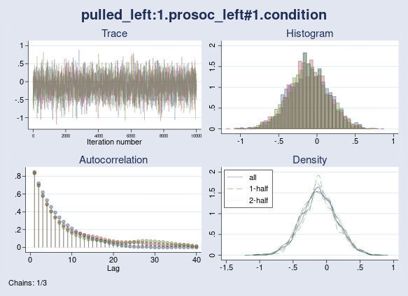
Let’s examine the convergence of the interplay between prosoc_left and situation graphically. I exploit the bayesgraph diagnostics command.
. bayesgraph diagnostics {pulled_left:1.prosoc_left#1.situation}
As we see, all chains combine effectively and exhibit comparable autocorrelation and density plots. We don’t have convergence considerations right here, which can be supported by the utmost Rc of 1.002 (< 1.1) from the earlier output.
When preliminary values disagree with the priors
As an example the impact of preliminary values on convergence, I run the mannequin utilizing random preliminary values drawn from the uniform(-100,-50) distribution, which strongly disagrees with the prior distribution of the regression parameters. I exploit the initall() possibility to use the identical initialization (sampling from the uniform(-100, -50) distribution) to all chains.
. bayes, prior({pulled_left:}, regular(0, 100))      ///
initall({pulled_left:} runiform(-100, -50))         ///
nchains(3) rseed(16) initsummary:                   ///
logit pulled_left 1.prosoc_left 1.prosoc_left#1.situation


Chain 1
  Burn-in ...
  Simulation ...

Chain 2
  Burn-in ...
  Simulation ...

Chain 3
  Burn-in ...
  Simulation ...

Mannequin abstract
------------------------------------------------------------------------------
Probability:
  pulled_left ~ logit(xb_pulled_left)

Priors:
              {pulled_left:1.prosoc_left} ~ regular(0,100)                  (1)
  {pulled_left:1.prosoc_left#1.situation} ~ regular(0,100)                  (1)
                      {pulled_left:_cons} ~ regular(0,100)                  (1)
------------------------------------------------------------------------------
(1) Parameters are components of the linear kind xb_pulled_left.

Preliminary values:
Chain 1:  {pulled_left:1.prosoc_left} -58.6507
{pulled_left:1.prosoc_left#1.situation} -95.4699 {pulled_left:_cons} -69.8725
Chain 2:  {pulled_left:1.prosoc_left} -71.6922
{pulled_left:1.prosoc_left#1.situation} -79.7403 {pulled_left:_cons} -89.2912
Chain 3:  {pulled_left:1.prosoc_left} -83.0878
{pulled_left:1.prosoc_left#1.situation} -73.2008 {pulled_left:_cons} -82.7553

Bayesian logistic regression                  Variety of chains    =          3
Random-walk Metropolis-Hastings sampling      Per MCMC chain:
                                                  Iterations      =     12,500
                                                  Burn-in         =      2,500
                                                  Pattern measurement     =     10,000
                                              Variety of obs       =        504
                                              Avg acceptance charge =      .2308
                                              Avg effectivity: min =     .04952
                                                              avg =     .05114
                                                              max =     .05339
Avg log marginal-likelihood = -350.48911      Max Gelman-Rubin Rc =       1.15

------------------------------------------------------------------------------
             |                                                Equal-tailed
 pulled_left |      Imply   Std. Dev.     MCSE     Median  [95% Cred. Interval]
-------------+----------------------------------------------------------------
1.prosoc_l~t |  .6805637   .2521363   .006541   .6655285   .2265225   1.189635
             |
 prosoc_left#|
   situation |
        1 1  | -.1545551    .273977   .006846  -.1557829   -.700246   .3686061
             |
       _cons |  .0272796   .1324386   .003403   .0262892   -.233117   .2766306
------------------------------------------------------------------------------
Word: Default preliminary values are used for a number of chains.
Word: There's a excessive autocorrelation after 500 lags in a minimum of one of many
      chains.
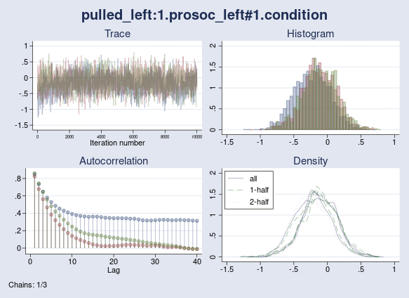
The utmost Rc is now 1.15 and is greater than the 1.1 threshold. I additionally see a excessive autocorrelation warning issued by the bayes:logit command. Lack of convergence is confirmed by the diagnostic plot of {pulled_left:1.prosoc_left} parameter, which reveals a random-walk hint plot and excessive autocorrelation for one of many chains.
. bayesgraph diagnostics {pulled_left:1.prosoc_left#1.situation}
Finally, I can nonetheless obtain convergence if I enhance the burn-in interval of the chains so all of them settle within the high-probability area of the posterior distribution. The purpose I need to make is that after you begin manipulating preliminary values, the default sampling settings could must be adjusted as effectively.
Random-intercept mannequin with bayesmh
I can additional elaborate the logistic regression mannequin by together with random-intercept coefficients for every particular person chimpanzee as recognized by the actor variable. I might match this mannequin utilizing bayes: melogit, however for better flexibility in specifying priors for random results, I’ll use the bayesmh command as a substitute. I will even use nonlinear specification for the regression part within the chance to match the precise specification utilized in McElreath (2016), 10.1.1. Within the new mannequin specification, the interplay between prosoc_left and situation is given by parameter bpC. The prior for the random intercepts {actors:i.actor} is regular with imply parameter {actor} and variance {sigma2_actor}. The latter is assigned an igamma(1, 1) hyperprior.
. bayesmh pulled_left = ({actors:}+({bp}+{bpC}*situation)*prosoc_left), ///
        redefine(actors:ibn.actor) chance(logit)                    ///
        prior({actors:i.actor}, regular({actor}, {sigma2_actor}))        ///
        prior({actor bp bpC}, regular(0, 100))                           ///
        prior({sigma2_actor}, igamma(1, 1))                             ///
        block({sigma2_actor}) nchains(3) rseed(101) dots


Chain 1
  Burn-in 2500 aaaaaaaaa1000aaaaaaaaa2000aa... achieved
  Simulation 10000 .........1000.........2000.........3000.........4000........
> .5000.........6000.........7000.........8000.........9000.........10000 achieved

Chain 2
  Burn-in 2500 aaaaaaaaa1000aaaaaaaaa2000aaaaa achieved
  Simulation 10000 .........1000.........2000.........3000.........4000........
> .5000.........6000.........7000.........8000.........9000.........10000 achieved

Chain 3
  Burn-in 2500 aaaaaaaaa1000aaaaaaaaa2000aaaaa achieved
  Simulation 10000 .........1000.........2000.........3000.........4000........
> .5000.........6000.........7000.........8000.........9000.........10000 achieved

Mannequin abstract
------------------------------------------------------------------------------
Probability:
  pulled_left ~ logit(xb_actors+({bp}+{bpC}*situation)*prosoc_left)

Priors:
  {actors:i.actor} ~ regular({actor},{sigma2_actor})                        (1)
          {bp bpC} ~ regular(0,100)

Hyperpriors:
         {actor} ~ regular(0,100)
  {sigma2_actor} ~ igamma(1,1)
------------------------------------------------------------------------------
(1) Parameters are components of the linear kind xb_actors.

Bayesian logistic regression                  Variety of chains    =          3
Random-walk Metropolis-Hastings sampling      Per MCMC chain:
                                                  Iterations      =     12,500
                                                  Burn-in         =      2,500
                                                  Pattern measurement     =     10,000
                                              Variety of obs       =        504
                                              Avg acceptance charge =      .3336
                                              Avg effectivity: min =     .03179
                                                              avg =     .04926
                                                              max =     .07257
Avg log marginal-likelihood = -283.00602      Max Gelman-Rubin Rc =      1.005

------------------------------------------------------------------------------
             |                                                Equal-tailed
             |      Imply   Std. Dev.     MCSE     Median  [95% Cred. Interval]
-------------+----------------------------------------------------------------
          bp |  .8250987   .2634764   .006958   .8253262   .3170529   1.351217
         bpC |  -.135104   .2896624   .006208  -.1332311  -.6942856   .4007747
       actor |  .3816366    .845064   .023025   .3478235  -1.207322   2.170198
sigma2_actor |  4.650094   3.831105   .124065   3.511577   1.149783    15.3841
------------------------------------------------------------------------------
Word: Default preliminary values are used for a number of chains.
I save the estimation outcomes of the brand new mannequin as model2.
. bayesmh, saving(model2)
notice: file model2.dta saved

. estimates retailer model2
Now, I can examine the 2 fashions utilizing the bayesstats ic command.
. bayesstats ic model1 model2

Bayesian data standards

---------------------------------------------------------
             |  Chains    Avg DIC  Avg log(ML)    log(BF)
-------------+-------------------------------------------
      model1 |       3   682.3504    -350.5063          .
      model2 |       3   532.2629    -283.0060    67.5003
---------------------------------------------------------
Word: Marginal chance (ML) is computed utilizing
      Laplace-Metropolis approximation.
As a result of each fashions have 3 chains, the command stories the common DIC and log-marginal chance throughout chains. The random-intercept mannequin is decidedly higher with respect to each Avg DIC and log(BF) standards. Using the better-fitting mannequin, nevertheless, doesn’t change the insignificance of the interplay time period bpC as measured by the posterior likelihood on the best facet of 0.
. bayestest interval {bpC}, decrease(0)

Interval checks     Variety of chains =         3
                   MCMC pattern measurement =    30,000

       prob1 : {bpC} > 0

-----------------------------------------------
             |      Imply    Std. Dev.      MCSE
-------------+---------------------------------
       prob1 |     .3227     0.46752   .0094796
-----------------------------------------------
Operating chains in parallel
Once you use the nchains() possibility wth bayesmh or bayes:, the chains are simulated sequentially, and the general simulation time is thus proportional to the variety of chains. Conditionally on the preliminary values, nevertheless, the chains are unbiased samples and may in precept be simulated in parallel. For good parallelization, a number of chains could be simulated within the time wanted to simulate only one chain.
The unofficial command bayesparallel permits a number of chains to be simulated in parallel. You’ll be able to set up the command utilizing internet set up.
. internet set up bayesparallel, from("http://www.stata.com/customers/nbalov")
bayesparallel is a prefix command that may be utilized to bayesmh and bayes:. bayesparallel implements parallelization by working a number of cases of Stata as separate processes. It has one notable possibility, nproc(#), to pick the variety of parallel processes for use for simulation. The default worth is 4, nproc(4). For extra consumer management, the command additionally supplies the stataexe() possibility for specifying the trail to the Stata executable file. For full description of the command, see the assistance file:
. assist bayesparallel
Let’s rerun model1 utilizing bayesparallel. I specify the nproc(3) possibility so that each one 3 chains are executed in parallel.
. bayesparallel, nproc(3):                                          ///
 bayes, prior({pulled_left:}, regular(0, 100)) nchains(3) rseed(16): ///
 logit pulled_left 1.prosoc_left 1.prosoc_left#1.situation

Simulating a number of chains ...

Completed.
As a result of the bayesparallel command doesn’t calculate any abstract statistics, I must recall bayes to see the outcomes.
. bayes

Mannequin abstract
------------------------------------------------------------------------------
Probability:
  pulled_left ~ logit(xb_pulled_left)

Priors:
              {pulled_left:1.prosoc_left} ~ regular(0,100)                  (1)
  {pulled_left:1.prosoc_left#1.situation} ~ regular(0,100)                  (1)
                      {pulled_left:_cons} ~ regular(0,100)                  (1)
------------------------------------------------------------------------------
(1) Parameters are components of the linear kind xb_pulled_left.

Bayesian logistic regression                  Variety of chains    =          3
Random-walk Metropolis-Hastings sampling      Per MCMC chain:
                                                  Iterations      =     12,500
                                                  Burn-in         =      2,500
                                                  Pattern measurement     =     10,000
                                              Variety of obs       =        504
                                              Avg acceptance charge =       .243
                                              Avg effectivity: min =     .06396
                                                              avg =     .07353
                                                              max =      .0854
Avg log marginal-likelihood =  -350.5063      Max Gelman-Rubin Rc =      1.001

------------------------------------------------------------------------------
             |                                                Equal-tailed
 pulled_left |      Imply   Std. Dev.     MCSE     Median  [95% Cred. Interval]
-------------+----------------------------------------------------------------
1.prosoc_l~t |  .6322682   .2278038   .005201   .6278013   .1925016   1.078073
             |
 prosoc_left#|
   situation |
        1 1  | -.1156446   .2674704   .005786  -.1126552   -.629691   .4001958
             |
       _cons |  .0438947   .1254382   .002478   .0448557  -.2092907   .2914614
------------------------------------------------------------------------------
The abstract outcomes match these of the primary run, the place the chains had been simulated sequentially, however the execution time was reduce in half. On my laptop working Stata/MP 16, the common simulation time for model1 was 5.4 seconds versus 2.7 seconds for the mannequin run with bayesparallel.
References
Brooks, S. P., and A. Gelman. 1998. Common strategies for monitoring convergence of iterative simulations. Journal of Computational and Graphical Statistics 7: 434–455. https://doi.org/10.1080/10618600.1998.10474787.
Gelman, A., J. B. Carlin, H. S. Stern, D. B. Dunson, A. Vehtari, and D. B. Rubin. 2013. Bayesian Knowledge Evaluation. third ed. Boca Raton, FL: Chapman & Corridor/CRC.
Gelman, A., and D. B. Rubin. 1992. Inference from iterative simulation utilizing a number of sequences. Statistical Science 7: 457–511. https://doi.org/10.1214/ss/1177011136.
McElreath, R. 2016. Statistical Rethinking: A Bayesian Course with Examples in R and Stan. Boca Raton, FL: CRC Press, Taylor and Francis Group.
Silk, J. a. a. 2005. Chimpanzees are detached to the welfare of unrelated group members. Nature 437: 1357–1359. https://doi.org/10.1038/nature04243.