KV Cache Optimization by way of Tensor Product Consideration

Desk of Contents

KV Cache Optimization by way of Tensor Product Consideration
Challenges with Grouped Question and Multi-Head Latent Consideration
Tensor Product Consideration (TPA)
PyTorch Implementation of Tensor Product Consideration (TPA)
Abstract
- Quotation Info

KV Cache Optimization by way of Tensor Product Consideration

Within the first two classes of this collection, we explored how trendy consideration mechanisms like Grouped Question Consideration (GQA) and Multi-Head Latent Consideration (MLA) can considerably cut back the reminiscence footprint of key-value (KV) caches throughout inference. GQA launched a intelligent technique to share keys and values throughout question teams, hanging a stability between expressiveness and effectivity. MLA took this additional by studying a compact latent area for consideration heads, enabling extra scalable inference with out sacrificing mannequin high quality.

Now, on this third installment, we dive into Tensor Product Consideration (TPA) — a novel strategy that reimagines the very construction of consideration representations. TPA leverages tensor decompositions to factorize queries, keys, and values into low-rank contextual elements, enabling a extremely compact and expressive illustration. This not solely slashes KV cache dimension but additionally integrates seamlessly with Rotary Positional Embeddings (RoPE), preserving positional consciousness.

On this tutorial, we’ll unpack the mechanics of TPA, its position in KV cache optimization, and the way it paves the best way for scalable, high-performance LLM inference.

This lesson is the final of a 3-part collection on LLM Inference Optimization — KV Cache:

To learn to optimize KV Cache utilizing Tensor Product Consideration, simply preserve studying.

In search of the supply code to this put up?

Leap Proper To The Downloads Part

Challenges with Grouped Question and Multi-Head Latent Consideration

Earlier than diving into Tensor Product Consideration (TPA), it’s necessary to know the restrictions of current KV cache optimization methods — significantly Grouped Question Consideration (GQA) and Multi-Head Latent Consideration (MLA) — and why they fall quick in scaling inference effectively.

Multi-Head Consideration (MHA)

Normal Multi-Head Consideration computes consideration independently throughout a number of heads, every with its personal set of question, key, and worth projections:

$text{Attention}(Q, K, V) = text{softmax}left(dfrac{QK^top}{sqrt{d_k}}right)V$

Every head $h$ makes use of its personal projections $W^K_h, W^V_h$ , leading to a KV cache dimension that scales linearly with the variety of heads and sequence size. Whereas expressive, this design incurs vital reminiscence overhead throughout inference.

Grouped Question Consideration (GQA)

GQA reduces KV cache dimension by sharing keys and values throughout teams of question heads. If $H$ is the variety of question heads and $G$ is the variety of key-value teams, then every group shares:

$K_g = W^K_g X, quad V_g = W^V_g X quad text{for } g = 1, dots, G$

This reduces cache dimension from $H times L$ to $G times L$ , the place $L$ is the sequence size. Nonetheless, GQA sacrifices flexibility — fewer key-value teams imply much less granularity in consideration — and sometimes requires architectural modifications to stability efficiency and effectivity.

Multi-Head Latent Consideration (MLA)

MLA, launched in DeepSeek-V2, compresses KV representations by projecting them right into a shared latent area:

$K' = W^K_{text{latent}} K, quad V' = W^V_{text{latent}} V$

This latent compression reduces reminiscence utilization, however integrating Rotary Positional Embeddings (RoPE) turns into problematic. RoPE usually operates per-head, and MLA’s shared latent area necessitates extra position-encoded parameters per head, complicating implementation and rising overhead.

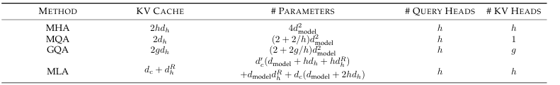
Desk 1 summarizes the KV cache dimension for the above consideration strategies as a perform of sequence size, mannequin hidden dimension, and variety of heads.

**Desk 1:** Comparability of various consideration mechanisms akin to MHA, GQA, MLA, and so on. (supply: Zhang et al., 2025).

Tensor Product Consideration (TPA)

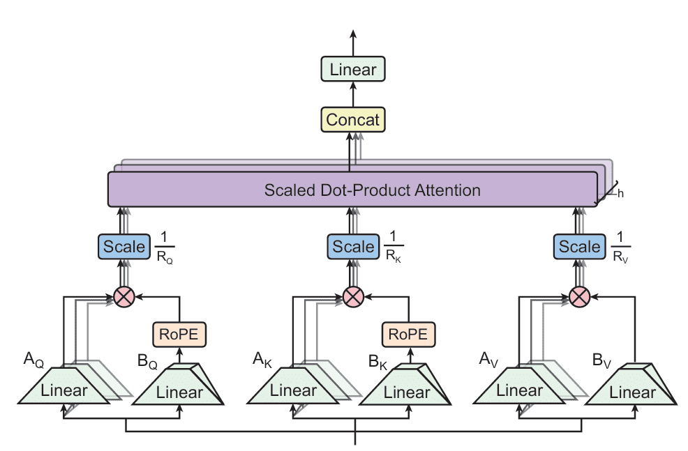
Tensor Product Consideration (TPA) is a novel consideration mechanism designed to handle the reminiscence bottlenecks of conventional multi-head consideration (MHA) throughout inference. In contrast to prior strategies that statically compress weights or share KV states throughout heads, TPA dynamically factorizes the activations — the queries, keys, and values — into low-rank elements. This permits compact, expressive representations that drastically cut back KV cache dimension whereas preserving mannequin high quality (Determine 1).

**Determine 1:** Illustration of Tensor Product Consideration (supply: Zhang et al., 2025).

TPA: Tensor Decomposition of Q, Ok, V

TPA replaces every head’s question, key, and worth vectors with a sum of tensor merchandise of latent elements derived from the token’s hidden state $(x_t)$ . Particularly, for every token $(t)$ :

$Q_t = dfrac{1}{R_Q} displaystylesum_{r=1}^{R_Q} A_Q^{(r)}(x_t) otimes B_Q^{(r)}(x_t) in mathbb{R}^{H times d_h}$

$K_t = dfrac{1}{R_K} displaystylesum_{r=1}^{R_K} A_K^{(r)}(x_t) otimes B_K^{(r)}(x_t) in mathbb{R}^{H times d_h}$

$V_t = dfrac{1}{R_V} displaystylesum_{r=1}^{R_V} A_V^{(r)}(x_t) otimes B_V^{(r)}(x_t) in mathbb{R}^{H times d_h}$

Right here:

$R_Q, R_K, R_V$ are the decomposition ranks
Every issue map $A^{(r)}(cdot), B^{(r)}(cdot)$ is a discovered perform of $x_t$
The outer product $otimes$ produces a rank-1 matrix per issue

This formulation permits every token’s KV state to be saved as a compact set of low-rank elements, lowering cache dimension to $mathcal{O}(T cdot R cdot (H + d_h))$ , the place $R = max(R_Q, R_K, R_V)$ .

Latent Issue Maps and Environment friendly Implementation

Every issue $A^{(r)}(cdot), B^{(r)}(cdot)$ is computed by way of linear projections from the token embedding:

$A_Q^{(r)}(x_t) = W^a_Q x_t in mathbb{R}^H, quad B_Q^{(r)}(x_t) = W^b_Q x_t in mathbb{R}^{d_h}$

To simplify implementation, the rank index is merged right into a single output dimension:

$A_Q(x_t) in mathbb{R}^{R_Q times H}, quad B_Q(x_t) in mathbb{R}^{R_Q times d_h}$

The ultimate question slice is computed as:

$Q_t = dfrac{1}{R_Q} A_Q(x_t)^top B_Q(x_t) in mathbb{R}^{H times d_h}$

Analogous definitions apply to $K_t$ and $V_t$ . This construction allows environment friendly batched computation and seamless integration into current Transformer pipelines.

Consideration Computation and RoPE Integration

TPA computes consideration scores utilizing the decomposed queries and keys:

$alpha_{ij} = text{softmax}left(dfrac{Q_i K_j^top}{sqrt{d_h}}right)$

And the output is:

$text{TPA}(Q, K, V)_i = displaystylesum_{j=1}^{T} alpha_{ij} V_j$

Crucially, Rotary Positional Embeddings (RoPE) are utilized on to the factorized elements:

$Q_t^{text{RoPE}} = displaystylesum_{r=1}^{R_Q} text{RoPE}(A_Q^{(r)}(x_t)) otimes B_Q^{(r)}(x_t)$

This preserves positional constancy with out requiring extra per-head parameters, in contrast to MLA.

Right here’s a transparent and concise subsection summarizing the KV caching and reminiscence discount advantages of Tensor Product Consideration:

KV Caching and Reminiscence Discount with TPA

In autoregressive decoding, customary multi-head consideration caches full key and worth tensors $K_t, V_t in mathbb{R}^{H times d_h}$ for every previous token $t$ , leading to a complete reminiscence price of $2T cdot H cdot d_h$ for a sequence of size $T$ . This grows linearly with each sequence size and head dimensionality, posing a significant scalability problem.

Tensor Product Consideration (TPA) addresses this by caching solely the factorized elements of keys and values. For every token $t$ , TPA shops:

$A_K(x_t) in mathbb{R}^{R_K times H} , B_K(x_t) in mathbb{R}^{R_K times d_h}$
$A_V(x_t) in mathbb{R}^{R_V times H} , B_V(x_t) in mathbb{R}^{R_V times d_h}$

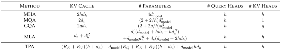
This reduces the per-token reminiscence price to (Desk 2):

$(R_K + R_V) cdot (H + d_h)$

In comparison with the usual price of $2 cdot H cdot d_h$ , the compression ratio turns into:

$dfrac{(R_K + R_V)(H + d_h)}{2H d_h}$

For typical head dimensions (e.g., $d_h = 64$ or $128$ ) and small ranks (e.g., $R_K, R_V = 1$ or $2$ ), TPA achieves substantial KV cache discount — usually by an order of magnitude. This permits longer sequence inference beneath fastened reminiscence budgets, making TPA particularly enticing for deployment in resource-constrained environments.

**Desk 2:** Comparability of various consideration mechanisms together with TPA (supply: Zhang et al., 2025).

PyTorch Implementation of Tensor Product Consideration (TPA)

On this part, we’ll stroll by means of the PyTorch implementation of the Tensor Product Consideration. We’ll break down the code into the important thing elements: the eye module, the transformer block, and the inference code.

Tensor Product Consideration with KV Caching

We start by implementing the core consideration mechanism within the MultiHeadTPAAttention class. This class inherits from torch.nn.Module and units up the mandatory layers for the eye calculation.

import torch
import torch.nn as nn
import time
import matplotlib.pyplot as plt
import math

class MultiHeadTPAAttention(nn.Module):
    def __init__(self, d_model=128*128, num_heads=128, R_q=12, R_kv=4):
        tremendous().__init__()
        self.d_model = d_model
        self.num_heads = num_heads
        self.R_q = R_q
        self.R_kv = R_kv
        self.head_dim = d_model // num_heads

        # Question projections
        self.Wq_a = nn.Linear(d_model, self.R_q*self.num_heads)
        self.Wq_b = nn.Linear(d_model, self.R_q*self.head_dim)

        # Key-value projections
        self.Wk_a = nn.Linear(d_model, self.R_kv*self.num_heads)
        self.Wk_b = nn.Linear(d_model, self.R_kv*self.head_dim)

        self.Wv_a = nn.Linear(d_model, self.R_kv*self.num_heads)
        self.Wv_b = nn.Linear(d_model, self.R_kv*self.head_dim)

        # Output projection
        self.Wo = nn.Linear(self.num_heads * self.head_dim, d_model)

    def ahead(self, x, kv_cache):
        batch_size, seq_len, d_model = x.form

        # Projections of enter into latent areas
        A_q, B_q = self.Wq_a(x), self.Wq_b(x)     # form: (batch_size, seq_len, q_latent_dim)
        A_k, B_k = self.Wk_a(x), self.Wk_b(x)   # form: (batch_size, seq_len, kv_latent_dim)
        A_v, B_v = self.Wv_a(x), self.Wv_b(x)   # form: (batch_size, seq_len, kv_latent_dim)

        A_q = A_q.view(batch_size, seq_len, self.num_heads, self.R_q)
        B_q = B_q.view(batch_size, seq_len, self.R_q, self.head_dim)

        A_k = A_k.view(batch_size, seq_len, self.num_heads, self.R_kv)
        B_k = B_k.view(batch_size, seq_len, self.R_kv, self.head_dim)

        A_v = A_v.view(batch_size, seq_len, self.num_heads, self.R_kv)
        B_v = B_v.view(batch_size, seq_len, self.R_kv, self.head_dim)


        # Append to cache
        kv_cache['A_k'] = torch.cat([kv_cache['A_k'], A_k], dim=1)
        kv_cache['B_k'] = torch.cat([kv_cache['B_k'], B_k], dim=1)

        kv_cache['A_v'] = torch.cat([kv_cache['A_v'], A_v], dim=1)
        kv_cache['B_v'] = torch.cat([kv_cache['B_v'], B_v], dim=1)

        # Increase KV heads to match question heads
        A_k = kv_cache['A_k']
        B_k = kv_cache['B_k']

        A_v = kv_cache['A_v']
        B_v = kv_cache['B_v']

        Q = torch.matmul(A_q, B_q)
        Ok = torch.matmul(A_k, B_k)
        V = torch.matmul(A_v, B_v)

        # Consideration rating, form: (batch_size, num_heads, seq_len, seq_len)
        scores = torch.matmul(Q.transpose(1, 2), Ok.transpose(1, 2).transpose(2, 3)) / math.sqrt(self.head_dim)
        # Consideration computation
        attn_weight = torch.softmax(scores, dim=-1)

        # Compute consideration output, form: (batch_size, seq_len, num_heads, head_dim)
        output = torch.matmul(attn_weight, V.transpose(1,2)).transpose(1,2).contiguous()
        # Concatenate the heads, then apply output projection
        output = self.Wo(output.view(batch_size, seq_len, -1))

        return output, kv_cache

On Strains 1-5, we import the mandatory PyTorch modules and different libraries for numerical operations and plotting. On Strains 7-28, we outline the MultiHeadTPAAttention class, initializing parameters such because the mannequin dimension (d_model), variety of consideration heads (num_heads), and the latent dimensions for queries (R_q) and keys/values (R_kv). We additionally outline linear layers that undertaking the enter into question, key, and worth elements within the latent area, in addition to an output projection layer.

On Strains 30-36, within the ahead methodology, we take the enter tensor x and the KV cache as arguments. We undertaking the enter x into latent representations A_q, B_q, A_k, B_k, A_v, and B_v utilizing the outlined linear layers. On Strains 34-45, we reshape these projected tensors to align with the multi-head consideration construction.

On Strains 49-53, we append the newly computed key and worth projections (A_k, B_k, A_v, B_v) to the prevailing KV cache. That is essential for environment friendly autoregressive inference, because it avoids recomputing the keys and values for earlier tokens. On Strains 56-64, we retrieve the up to date key and worth projections from the cache after which compute the Question (Q), Key (Ok), and Worth (V) tensors by multiplying their respective A and B elements.

On Strains 67-69, we calculate the eye scores by taking the dot product of the Question and Key tensors, scaled by the sq. root of the top dimension. We then apply the softmax perform to acquire the eye weights. Lastly, on Strains 72-76, we compute the eye output by multiplying the eye weights with the Worth tensor, reshape the output, and apply the ultimate output projection. The perform returns the eye output and the up to date KV cache.

Transformer Block

Subsequent, we implement a easy Transformer block that includes the Tensor Product Consideration module.

class TransformerBlock(nn.Module):
    def __init__(self,  d_model=128*128, num_heads=128, R_q=12, R_kv=4):
        tremendous().__init__()
        self.attn = MultiHeadTPAAttention(d_model, num_heads, R_q, R_kv)
        self.norm1 = nn.LayerNorm(d_model)
        self.ff = nn.Sequential(
            nn.Linear(d_model, d_model * 4),
            nn.ReLU(),
            nn.Linear(d_model * 4, d_model)
        )
        self.norm2 = nn.LayerNorm(d_model)

    def ahead(self, x, kv_cache):
        attn_out, kv_cache = self.attn(x, kv_cache)
        x = self.norm1(x + attn_out)
        ff_out = self.ff(x)
        x = self.norm2(x + ff_out)
        return x, kv_cache

On Strains 77-87, we outline the TransformerBlock class, which incorporates an occasion of our MultiHeadTPAAttention module, two situations of layer normalization (norm1 and norm2), and a feed-forward community (ff). The feed-forward community consists of two linear layers with a ReLU activation in between.

On Strains 89-94, within the ahead methodology, the enter x first passes by means of the eye layer together with the KV cache. The eye layer’s output is then added to the unique enter (a residual connection) and normalized. That is adopted by the feed-forward community, and one other residual connection and layer normalization. The perform returns the output of the transformer block and the up to date KV cache.

Inferencing Code

Subsequent, we now have the run_inference perform, which simulates the autoregressive era course of.

def run_inference(block):
    d_model = block.attn.d_model
    num_heads = block.attn.num_heads
    kv_latent_dim = block.attn.R_kv

    seq_lengths = listing(vary(1, 50, 10))
    kv_cache_sizes = []
    inference_times = []

    kv_cache = {
        'A_k': torch.empty(1, 0, num_heads, kv_latent_dim),
        'B_k': torch.empty(1, 0, kv_latent_dim, d_model // num_heads),
        'B_v': torch.empty(1, 0, kv_latent_dim, d_model // num_heads),
        'A_v': torch.empty(1, 0, num_heads, kv_latent_dim),
    }

    for seq_len in seq_lengths:
        x = torch.randn(1, 1, d_model)  # One token at a time
        begin = time.time()
        o, kv_cache = block(x, kv_cache)
        finish = time.time()
        dimension = kv_cache['A_k'].numel() + kv_cache['B_v'].numel() + kv_cache['B_k'].numel() + kv_cache['A_v'].numel()
        kv_cache_sizes.append(dimension)
        inference_times.append(finish - begin)

    return seq_lengths, kv_cache_sizes, inference_times

The run_inference perform (Strains 95-102) simulates the autoregressive era means of a Transformer block. We initialize an empty KV cache (Strains 104-109) that shops the keys and values from earlier tokens. We then iterate by means of a variety of sequence lengths (Line 111), simulating the era of 1 token at a time (Line 112). For every token, we go it by means of the TransformerBlock (Line 114), which updates the KV cache. We measure the time taken for every step and the dimensions of the KV cache (Strains 115 and 116).

After processing all of the tokens for a given sequence size, we document the KV cache dimension and inference time. This course of is repeated for various sequence lengths, permitting us to look at how the KV cache dimension and inference time change because the sequence grows. Lastly, we return the collected information for plotting and evaluation (Line 120).

Experimentation

plt.determine(figsize=(12, 5))
plt.subplot(1, 2, 1)

for latent_dim in [2, 4, 8, 16, 32]:
  mla_block = TransformerBlock(d_model=4096, num_heads=32, R_q=12, R_kv=latent_dim)
  seq_lengths, sizes, occasions = run_inference(mla_block)
  plt.plot(seq_lengths, sizes, label="TPA R_kv dim : {}".format(latent_dim))

plt.xlabel("Generated Tokens")
plt.ylabel("KV Cache Dimension")
plt.title("KV Cache Development")
plt.legend()

plt.subplot(1, 2, 2)
for latent_dim in [2, 4, 8, 16, 32]:
    mla_block = TransformerBlock(d_model=4096, num_heads=32, R_q=12, R_kv=latent_dim)
    seq_lengths, sizes, occasions = run_inference(mla_block)
    plt.plot(seq_lengths, occasions, label="TPA R_kv dim : {}".format(latent_dim))


plt.xlabel("Generated Tokens")
plt.ylabel("Inference Time (s)")
plt.title("Inference Velocity")

plt.legend()

plt.tight_layout()
plt.present()

Output:

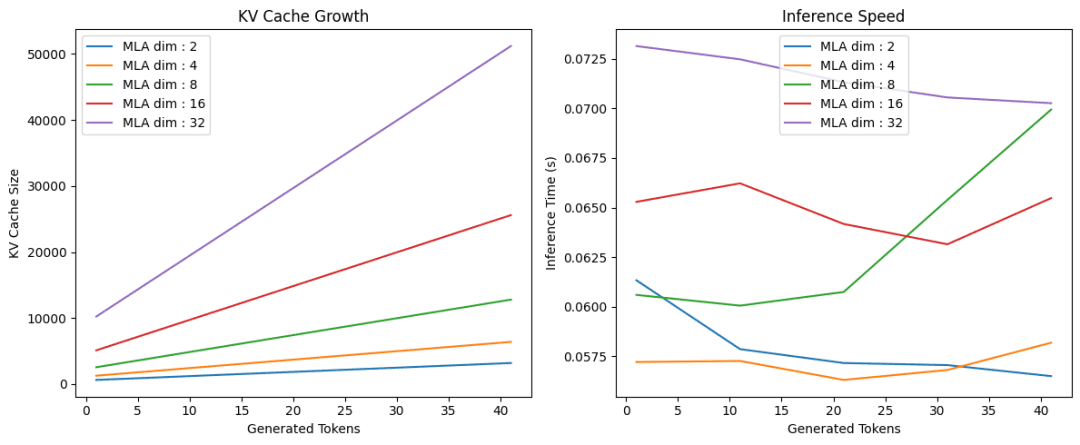
**Determine 2:** Discount in KV Cache dimension through the use of Tensor Product consideration of assorted latent dimensions (supply: picture by the writer).

On this code (Strains 121-148), we conduct experiments to research the efficiency of the tensor product consideration mechanism throughout completely different KV latent dimensions. We arrange a determine with two subplots (Strains 121 and 122) to visualise the outcomes. We then iterate by means of an inventory of various latent dimensions (Line 124). For every latent dimension, we create a TransformerBlock occasion with the required d_model, num_heads, R_q, and the present latent_dim for R_kv (Line 125). We then name the run_inference perform (Line 126) with this block to get the sequence lengths, KV cache sizes, and inference occasions.

We then plot the KV cache sizes towards the generated tokens (sequence lengths) on the primary subplot (Strains 127-132) and the inference occasions towards the generated tokens on the second subplot (Strains 138-143). This permits us to match how completely different latent dimensions have an effect on the KV cache development and inference pace (Determine 2).

What’s subsequent? We advocate PyImageSearch College.

Course data:
86+ whole lessons • 115+ hours hours of on-demand code walkthrough movies • Final up to date: December 2025
★★★★★ 4.84 (128 Rankings) • 16,000+ College students Enrolled

I strongly consider that for those who had the appropriate instructor you possibly can grasp pc imaginative and prescient and deep studying.

Do you assume studying pc imaginative and prescient and deep studying must be time-consuming, overwhelming, and complex? Or has to contain complicated arithmetic and equations? Or requires a level in pc science?

That’s not the case.

All you must grasp pc imaginative and prescient and deep studying is for somebody to elucidate issues to you in easy, intuitive phrases. And that’s precisely what I do. My mission is to vary schooling and the way complicated Synthetic Intelligence subjects are taught.

If you happen to’re critical about studying pc imaginative and prescient, your subsequent cease ought to be PyImageSearch College, essentially the most complete pc imaginative and prescient, deep studying, and OpenCV course on-line right now. Right here you’ll learn to efficiently and confidently apply pc imaginative and prescient to your work, analysis, and tasks. Be part of me in pc imaginative and prescient mastery.

Inside PyImageSearch College you will discover:

&verify; 86+ programs on important pc imaginative and prescient, deep studying, and OpenCV subjects
&verify; 86 Certificates of Completion
&verify; 115+ hours hours of on-demand video
&verify; Model new programs launched frequently, guaranteeing you’ll be able to sustain with state-of-the-art methods
&verify; Pre-configured Jupyter Notebooks in Google Colab
&verify; Run all code examples in your internet browser — works on Home windows, macOS, and Linux (no dev atmosphere configuration required!)
&verify; Entry to centralized code repos for all 540+ tutorials on PyImageSearch
&verify; Straightforward one-click downloads for code, datasets, pre-trained fashions, and so on.
&verify; Entry on cellular, laptop computer, desktop, and so on.

Click on right here to affix PyImageSearch College

Abstract

On this third installment of our collection on LLM Inference Optimization, we delve into Tensor Product Consideration (TPA), a novel strategy to reimagining consideration representations. We discover how TPA leverages tensor decompositions to factorize queries, keys, and values into low-rank contextual elements. This methodology considerably reduces KV cache dimension and seamlessly integrates with Rotary Positional Embeddings (RoPE), sustaining positional consciousness with out extra per-head parameters.

We study the mechanics of TPA, contrasting it with the restrictions of current KV cache optimization methods akin to Grouped Question Consideration (GQA) and Multi-Head Latent Consideration (MLA). Whereas GQA shares keys and values throughout question teams and MLA compresses KV representations right into a shared latent area, TPA dynamically factorizes activations, storing KV states as compact units of low-rank elements. This leads to a reminiscence price that scales extra effectively with sequence size and head dimensionality.

In the end, we display how TPA paves the best way for scalable, high-performance LLM inference by addressing the reminiscence bottlenecks of conventional multi-head consideration. By caching solely the factorized elements of keys and values, TPA presents a extra memory-efficient resolution for autoregressive decoding.

Quotation Info

Mangla, P. “KV Cache Optimization by way of Tensor Product Consideration,” PyImageSearch, P. Chugh, S. Huot, A. Sharma, and P. Thakur, eds., 2025, https://pyimg.co/6ludn

@incollection{Mangla_2025_kv-cache-optimization-via-tensor-product-attention,
  writer = {Puneet Mangla},
  title = {{KV Cache Optimization by way of Tensor Product Consideration}},
  booktitle = {PyImageSearch},
  editor = {Puneet Chugh and Susan Huot and Aditya Sharma and Piyush Thakur},
  12 months = {2025},
  url = {https://pyimg.co/6ludn},
}

To obtain the supply code to this put up (and be notified when future tutorials are revealed right here on PyImageSearch), merely enter your electronic mail deal with within the type under!

Obtain the Supply Code and FREE 17-page Useful resource Information

Enter your electronic mail deal with under to get a .zip of the code and a FREE 17-page Useful resource Information on Laptop Imaginative and prescient, OpenCV, and Deep Studying. Inside you will discover my hand-picked tutorials, books, programs, and libraries that can assist you grasp CV and DL!

The put up KV Cache Optimization by way of Tensor Product Consideration appeared first on PyImageSearch.

KV Cache Optimization by way of Tensor Product Consideration

KV Cache Optimization by way of Tensor Product Consideration

In search of the supply code to this put up?

Challenges with Grouped Question and Multi-Head Latent Consideration

Multi-Head Consideration (MHA)

Grouped Question Consideration (GQA)

Multi-Head Latent Consideration (MLA)

Tensor Product Consideration (TPA)

TPA: Tensor Decomposition of Q, Ok, V

Latent Issue Maps and Environment friendly Implementation

Consideration Computation and RoPE Integration

KV Caching and Reminiscence Discount with TPA

PyTorch Implementation of Tensor Product Consideration (TPA)

Tensor Product Consideration with KV Caching

Transformer Block

Inferencing Code

Experimentation

What’s subsequent? We advocate PyImageSearch College.

Abstract

Quotation Info

Obtain the Supply Code and FREE 17-page Useful resource Information

Related Articles

An introduction to the lasso in Stata

The Greatest Net Scraping APIs for AI Fashions in 2026

IT Leaders Quick-5: Craig Williams, Ciena

Latest Articles

An introduction to the lasso in Stata

The Greatest Net Scraping APIs for AI Fashions in 2026

IT Leaders Quick-5: Craig Williams, Ciena

Posit AI Weblog: Practice in R, run on Android: Picture segmentation with torch

Your Pixel can now do away with HDR photos and movies, this is how