
The only model of the central restrict theorem (CLT) says that if (X_1, dots, X_n) are iid random variables with imply (mu) and finite variance (sigma^2)
[
frac{bar{X}_n – mu}{sigma/sqrt{n}} rightarrow_d N(0,1)
]
the place (bar{X}_n = frac{1}{n} sum_{i=1}^n X_i). In different phrases, if (n) is sufficiently giant, the pattern imply is roughly usually distributed with imply (mu) and variance (sigma^2/n), whatever the distribution of (X_1, dots, X_n). This can be a fairly spectacular outcome! It’s so spectacular, in reality, that college students encountering it for the primary time are normally somewhat cautious. I’m sometimes requested “however how giant is sufficiently giant?” or “how do we all know when the CLT will present a superb approximation?” My reply is disappointing: with out some further details about the distribution from which (X_1, dots, X_n) have been drawn, we merely can’t say how giant a pattern is giant sufficient for the CLT work nicely. At this level, somebody invariably volunteers “however in my highschool statistics course, we realized that (n = 30) is large enough for the CLT to carry!”
I’ve at all times been shocked by the prevalence of the (n geq 30) dictum. It even seems in Charles Wheelan’s Bare Statistics, an in any other case glorious e-book that I assign as summer season studying for our incoming economics undergraduates: “as a rule of thumb, the pattern dimension have to be no less than 30 for the central restrict theorem to carry true.” On this submit I’d prefer to set the file straight: (ngeq 30) is neither vital nor enough for the CLT to offer a superb approximation, as we’ll see by inspecting two easy examples. Alongside the way in which, we’ll find out about two helpful instruments for visualizing and evaluating distributions: the empirical cdf, and quantile-quantile plots.
A pattern dimension of thirty isn’t vital.
We’ll begin by displaying that the CLT can work extraordinarily nicely even when (n) is way smaller than (30) and the random variables that we common are removed from usually distributed themselves. Alongside the way in which we’ll study in regards to the empirical CDF and quantile-quantile plots, two extraordinarily helpful instruments for evaluating likelihood distributions.
Informally talking, a Uniform((0,1)) random variable is equally prone to tackle any steady worth within the vary ([0,1]). Right here’s a histogram of 1000 random attracts from this distribution:
# set the seed to get the identical attracts I did
set.seed(12345)
hist(runif(1000), xlab = '', freq = FALSE,
     most important = 'Histogram of 1000 Uniform(0,1) Attracts')
This distribution clearly isn’t regular!
Certainly, its likelihood density operate is (f(x) = 1) for (x in [0,1]).
This can be a flat line reasonably than a bell curve.
But when we common even a comparatively small variety of Uniform((0,1)) attracts, the outcome can be extraordinarily shut to normality. To see that that is true, we’ll perform a simulation through which we draw (n) Uniform((0,1)) RVs, calculate their pattern imply, and retailer the outcome. Repeating this numerous occasions permits us to approximate the sampling distribution of (bar{X}_n). I’ll begin by writing a operate get_unif_sim that takes a single argument n. This operate returns the pattern imply of n Uniform((0,1)) attracts:
get_unif_sim <- operate(n) {
  sims <- runif(n)
  xbar <- imply(sims)
  return(xbar)
}
Subsequent I’ll use the replicate operate to name get_unif_sim numerous occasions, nreps, and retailer the outcomes as a vector referred to as xbar_sims. Right here I’ll take (n = 10) normal uniform attracts, blatantly violating the (n geq 30) rule-of-thumb:
set.seed(12345)
nreps <- 1e5 # scientific notation for 100,000
xbar_sims <- replicate(nreps, get_unif_sim(10))
hist(xbar_sims, xlab = '', freq = FALSE,
     most important = 'Sampling Dist. of Pattern Imply of 10 Uniform(0,1) Attracts')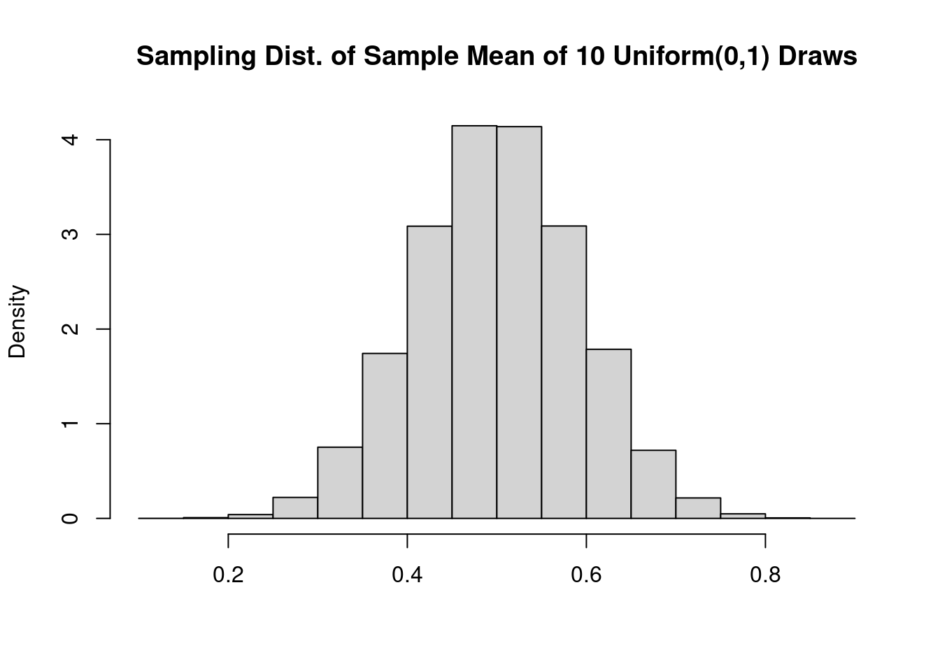
A phenomenal bell curve! This definitely appears regular, however histograms may be difficult to interpret. Their form relies on what number of bins we use to make the plot, one thing that may be tough to decide on nicely in observe. Within the following two sections, we’ll as an alternative examine distribution capabilities and quantiles.
The Empirical CDF
If (X sim) Uniform((0,1)), then (mathbb{E}(X) = 1/2) and (textual content{Var}(X) = 1/12), which follows from (mathbb{E}[X^2]=1/3) and the definition of variance. For (n = 10),
[
frac{sigma}{sqrt{n}} = frac{1}{sqrt{12}} cdot frac{1}{sqrt{10}} = frac{1}{sqrt{120}}
]
so if the CLT gives a superb approximation on this instance, we should always discover that
[
frac{bar{X}_n – 1/2}{1/sqrt{120}} = sqrt{120} (bar{X}_n – 1/2) approx N(0,1)
]
within the sense that that the cumulative distribution operate (CDF) of (sqrt{120} (bar{X}_n – 1/2)), name it (F), is roughly equal to the usual regular CDF pnorm(). An apparent technique to see if this holds is to plot (F) towards pnorm() and see how they examine. Any longer, we’ll be working with the z-scores of xbar_sims reasonably than the uncooked simulation values themselves, so we’ll begin by setting up them, subtracting the inhabitants imply and dividing by the inhabitants normal deviation:
z <- (xbar_sims - 1/2) / (1 / sqrt(120))We haven’t labored out an expression for the operate (F), however we are able to approximate it utilizing our simulation attracts xbar_sims. We do that by calculating the empirical CDF of our centered and standardized simulation attracts z. Recall that if (Z) is a random variable, its CDF (F) is outlined as (F(t) = mathbb{P}(Z leq t)). Given numerous noticed random attracts (z_1, dots, z_J) from the distribution of (Z), we are able to approximate (mathbb{P}(Z leq t)) by calculating the fraction of noticed attracts lower than or equal to (t). In different phrases
[
mathbb{P}(Z leq t) approx frac{1}{J}sum_{j=1}^J mathbf{1}{z_j leq t}
]
the place (mathbf{1}{z_j leq t }) is the indicator operate: it equals one if (z_j) is lower than or equal to the brink (t) and 0 in any other case. The pattern common on the right-hand aspect of the previous expression known as the empirical CDF. It makes use of empirical information–on this case our simulation attracts (z_j)–to approximate the unknown CDF. By growing the variety of random attracts (J) that we use, we are able to make this approximation as correct as we like. For instance, we don’t know the precise worth of (F(0)), the likelihood that (Z leq 0). However utilizing our simulated values z from above, we are able to approximate it as
imply(z <= 0)## [1] 0.49993and if we wished to the likelihood that (Z leq 2), we might approximate this as
imply(z <= 2)## [1] 0.97797Up to now so good: these values agree with pnorm(0), which equals 0.5, and pnorm(2), which is roughly 0.9772.
However we’ve solely checked out two values of (t).
Whereas we might proceed making an attempt further values one by one, it’s a lot quicker to make use of R’s built-in operate for computing an empirical cdf, ecdf(). First we cross our simulated z-scores z into ecdf() operate to calculate the empirical CDF and plot the outcome. Subsequent we overlay some factors from the usual regular CDF, pnorm in blue for comparability:
z <- sqrt(120) * (xbar_sims - 1/2)
plot(ecdf(z), xlab = 't', ylab = 'F(t)', most important = 'F(t) versus pnorm(t)')
tseq <- seq(-4, 4, by = 0.2)
factors(tseq, pnorm(tseq), col = 'blue')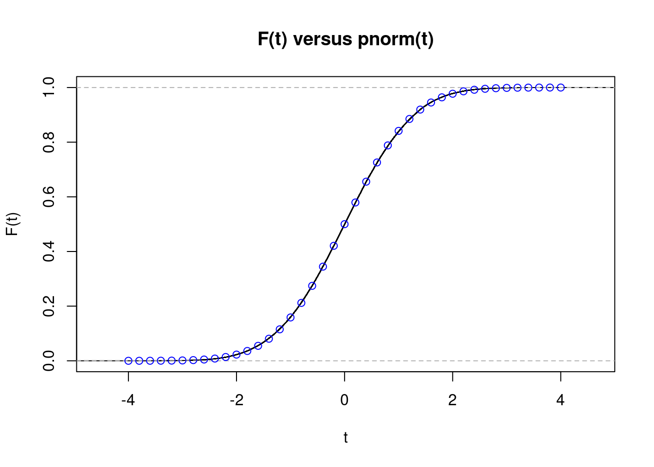
The match is nearly excellent, regardless of (n=10) being far under 30. This type of plot is way more informative than the histogram from above, however it could possibly nonetheless be a bit tough to learn. When setting up confidence intervals or calculating p-values it’s chances within the tails of the distribution that matter most, i.e. values of (t) which can be removed from zero within the plot. Ideally, we’d like a plot that makes any discrepancies within the tails soar out at us. That’s exactly what we’ll assemble subsequent.
Quantile-Quantile Plots
Up to now we’ve seen that the histogram of xbar_sims is bell-shaped, and that the empirical CDF of sqrt(120) * (xbar_sims - 0.5) is well-approximated by the usual regular CDF pnorm(). If you happen to’re nonetheless not satisfied that the CLT can work completely nicely with (n = 10), the ultimate plot that we’ll make ought to dispel any remaining doubts.
As its identify suggests, a quantile-quantile plot compares the quantiles of two likelihood distributions. However reasonably than evaluating two quantile capabilities plotted towards (p), it compares the quantiles of two distributions plotted towards one another. This can be a bit complicated the primary time you encounter it, so we’ll take issues step-by-step.
If our simulated z-scores from above are well-approximated by a regular regular distribution, then their median must be near that of a regular regular random variable, i.e. zero. That is certainly the case:
median(z)## [1] 0.0001169817But it surely’s not simply the medians that must be shut to one another: all the quantiles must be. So now let’s take a look at the Twenty fifth-percentile and Seventy fifth-percentile as nicely. Somewhat than computing them one-by-one, we are able to generate them in a single batch by first organising a vector p of chances and utilizing rbind to print the leads to a handy format
p <- c(0.25, 0.5, 0.75)
rbind(regular = qnorm(p), simulation =  quantile(z, probs = p))
## 25% 50% 75%
## regular -0.6744898 0.0000000000 0.6744898
## simulation -0.6779843 0.0001169817 0.6791994This appears good as nicely.
If we need to examine quantiles over a finer grid of values for p, it’s extra handy to make a plot reasonably than a desk. Suppose that we deal with the values qnorm as an (x)-coordinate and the quantiles of z as a (y)-coordinate. If the CLT is giving us a superb approximation, then we should always have (x approx y) and the entire factors ought to fall close to the 45-degree line. That is certainly what we observe:
p <- seq(from = 0.05, to = 0.95, by = 0.05)
x <- qnorm(p)
y <- quantile(z, probs = p)
plot(x, y, xlab = 'std. regular quantiles', ylab = 'quantiles of z')
abline(0, 1) # plot the 45-degree line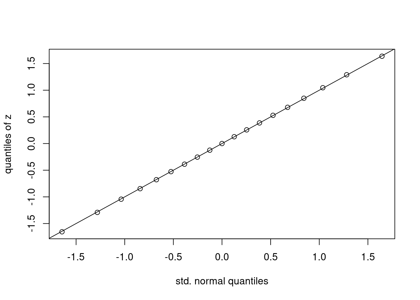
The plot that we have now simply made known as a regular quantile-quantile plot. It’s constructed as follows:
- Arrange a vector
pof chances. - Calculate the corresponding quantiles of a regular regular RV,
qnorm(p). Name these (x). - Calculate the corresponding quantiles of your information,
quantile(your_data_here, probs = p). Name them (y). - Plot (y) towards (x).
If the factors all fall on a line, then the quantiles of the noticed information agree with these of some regular distribution, though maybe not a regular regular. If we standardize the info earlier than making such a plot, as we did to assemble z above, the related line with be the 45-degree line. If not, it is going to be a distinct line however the interpretation stays the identical The simplest technique to make a standard quantile-quantile plot in R is by utilizing the operate qqnorm adopted by qqline. We might do that both utilizing the centered and standardized simulation attracts z or the unique attracts xbar_sims
par(mfrow = c(1, 2))
qqnorm(z, ylab = 'Quantiles of z')
qqline(z)
qqnorm(xbar_sims, ylab = 'Quantiles of xbar_sims')
qqline(xbar_sims)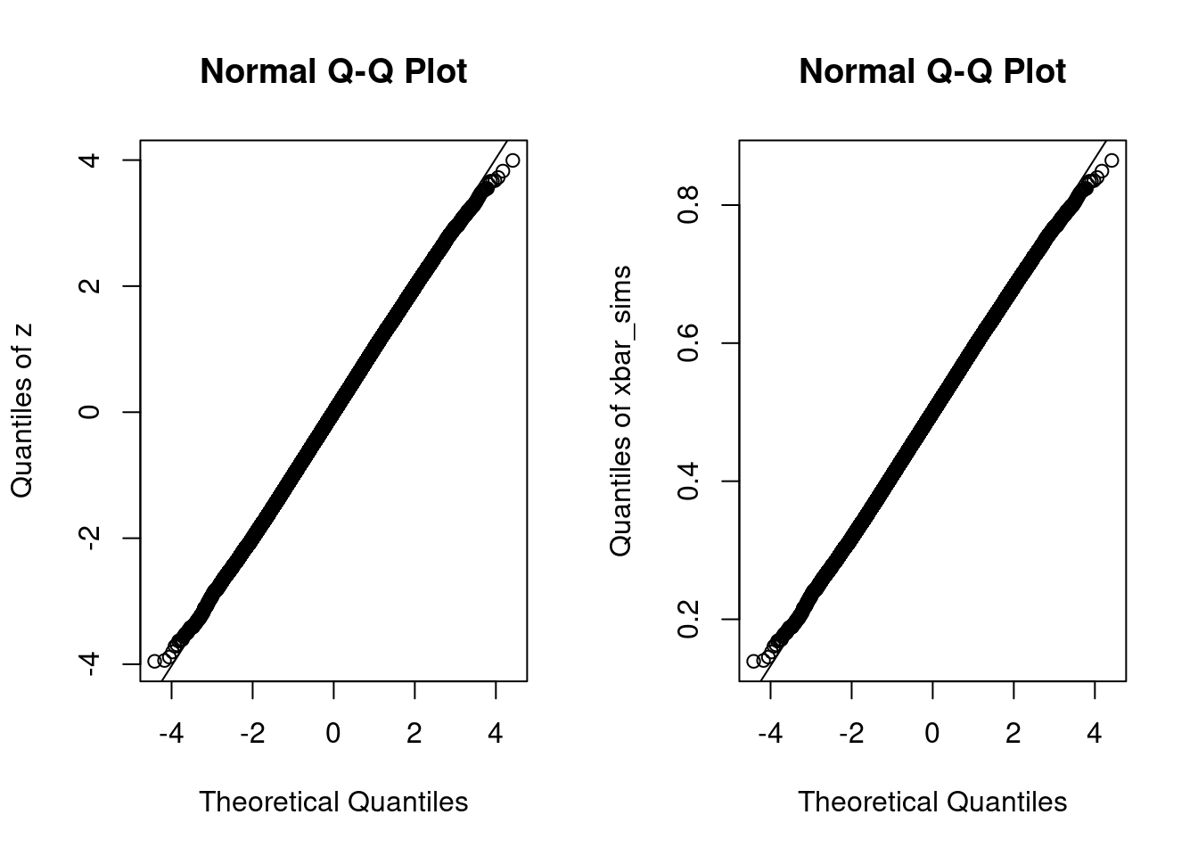
par(mfrow = c(1, 1))The one distinction between these two plots is the dimensions of the (y)-axis. The plot that makes use of the unique simulation attracts xbar_sims has a (y)-axis that runs between (0.1) and (0.9) as a result of the pattern common of (textual content{Uniform}(0,1)) random variables should lie throughout the interval ([0,1]). In distinction, the corresponding (z)-scores lie within the vary ([-4,4]). For (x)-values between (-3) and (3), we are able to’t even see the road generated by qqline: the quantiles of our simulation attracts are extraordinarily near these of a standard distribution. Exterior of this vary, nevertheless, we see that the black circles curve away from the road. For values of (x) round (-4), the quantiles of z are above these of a regular regular, i.e. shifted to the proper. For values of (x) round (4), the image is reversed: the quantiles of z are under these of a regular regular, i.e. shifted to the left. Which means z has lighter tails than a regular regular: it’s a bit much less prone to yield extraordinarily giant constructive or destructive values, for instance
cbind(simulation = quantile(z, 0.0001), regular = qnorm(0.0001))## simulation regular
## 0.01% -3.563576 -3.719016This makes excellent sense. A normal regular can tackle arbitrarily giant values, whereas the pattern imply of ten uniforms is essentially bounded above by (1). So if you wish to perform a (0.01%) check ((alpha = 0.0001)), the approximation offered by the CLT received’t fairly lower it with (n = 10) on this instance. However for any typical significance stage, it’s practically excellent:
p <- c(0.01, 0.025, 0.05, 0.1)
rbind(regular = qnorm(p), simulation = quantile(z, prob = p))
## 1% 2.5% 5% 10%
## regular -2.326348 -1.959964 -1.644854 -1.281552
## simulation -2.302793 -1.958568 -1.654508 -1.290797A pattern dimension of thirty isn’t enough.
Now suppose that (n = 100) and (X_1, dots X_n sim) iid Bernoulli((1/60)). What’s the CDF of (bar{X}_n)? Somewhat than approximating the reply to this query by simulation, as we did within the uniform instance from above, we’ll work out the precise outcome and examine it to the approximation offered by the CLT. If (X_1, dots, X_n sim) iid Bernoulli((p)), then by definition the sum (S_n = sum_{i=1}^n X_i) follows a Binomial((n,p)) distribution. The likelihood mass operate and CDF of this distribution can be found in R through the dbinom() and pbinom() instructions. So what about (bar{X}_n)? Discover that
[
mathbb{P}(bar{X}_n = x) = mathbb{P}(S_n/n = x) = mathbb{P}(S_n = nx)
]
Thus, if (f(s) = mathbb{P}(S_n = s)) is the pmf of (S_n) for (s in {0, 1, dots n}), it follows that (f(nx)) is the pmf of (bar{X}_n) for (x in {0, 1/n, 2/n, dots, 1}). Which means we are able to use dbinom to plot the precise sampling distribution of (bar{X}_n) when (n = 100) and (p = 1/60) as follows
n <- 100
p <- 1/60
x <- seq(from = 0, to = 1, by = 1/n)
P_x_bar <- dbinom(n * x, dimension = n, prob = p)
plot(x, P_x_bar, kind = 'h', xlim = c(0, 0.1), ylab = 'pmf of Xbar',
     lwd = 2, col = 'blue')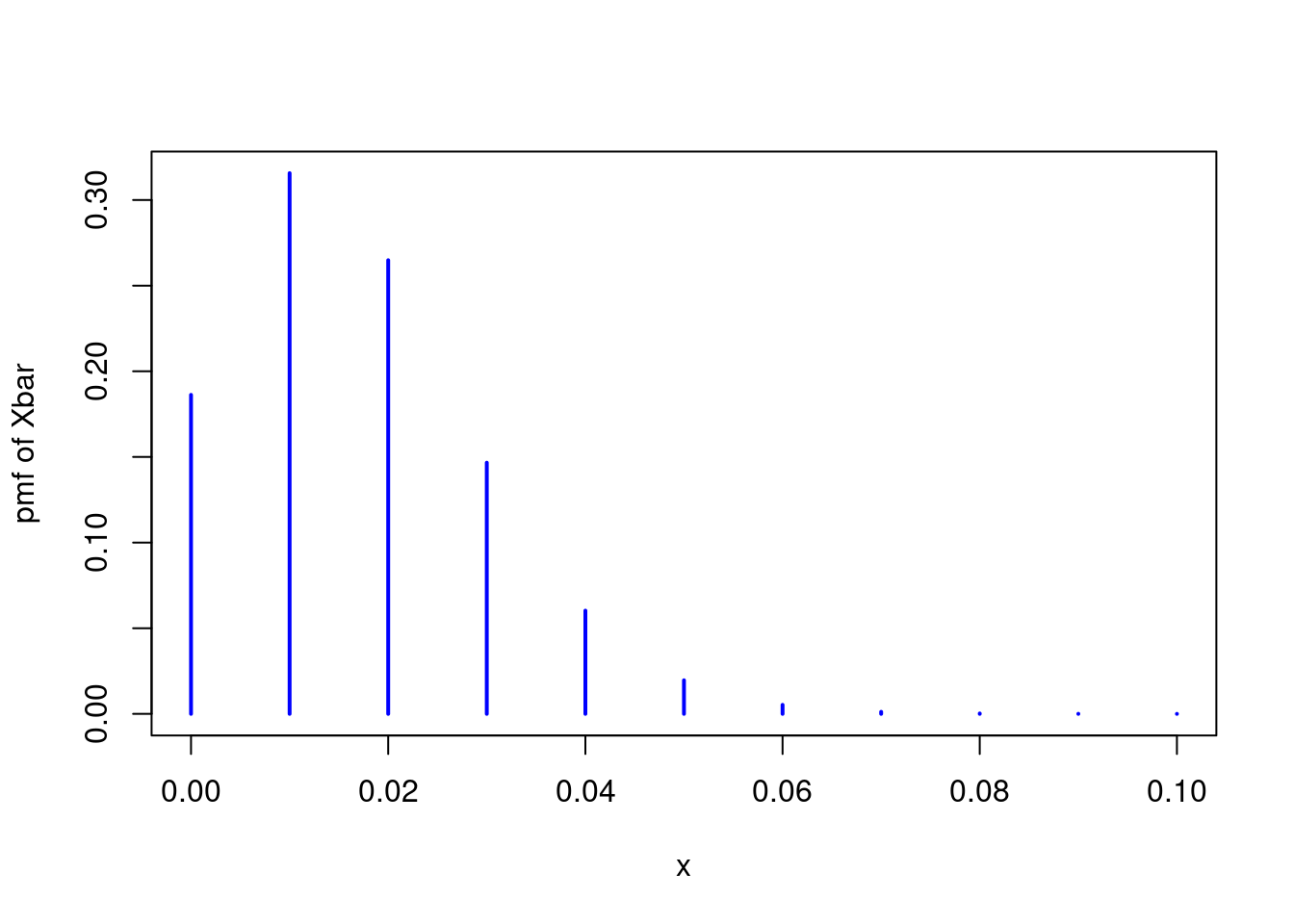
The result’s far from a standard distribution. Not solely is it noticeably discrete, it’s also critically uneven. One other technique to see that is by inspecting the CDF. If the central restrict theorem is working nicely on this instance, we should always have (bar{X}_n approx Nbig(p, p(1 – p)/nbig)). Extending the concept from above, we are able to plot the precise CDF of (bar{X}_n) utilizing the binomial CDF pbinom() and examine it to the approximation steered by the CLT:
x <- seq(-0.02, 0.08, by = 0.001)
F_x_bar <- pbinom(n * x, dimension = n, prob = p)
F_clt <- pnorm(x, p, sqrt(p * (1 - p) / n))
plot(x, F_x_bar, kind = 's', ylab = '', lwd = 2, col = 'blue')
factors(x, F_clt, kind = 'l', lty = 2, lwd = 2, col = 'pink')
legend('topleft', legend = c('Actual', 'CLT'), col = c('blue', 'pink'),
       lty = 1:2, lwd = 2)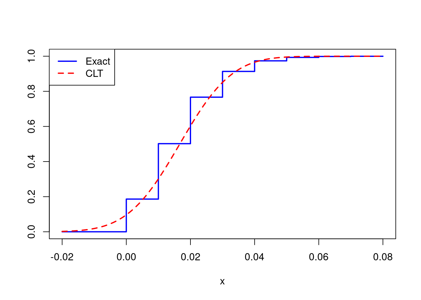
The approximation is noticeably poor, however is the issue severe sufficient to have an effect on any inferences we would hope to attract? Suppose we wished to assemble a 95% confidence interval for (p). The textbook strategy, primarily based on the CLT, would have us report (widehat{p} pm 1.96 occasions sqrt{widehat{p}(1 – widehat{p})/n}) the place (widehat{p}) is the pattern proportion, i.e. (bar{X}_n). Let’s arrange somewhat simulation experiment to see how nicely this interval performs when (n = 100) and (p = 1/60).
# Simulate 5000 attracts for phat
# with p = 1/60, n = 100
set.seed(54321)
draw_sim_phat <- operate(p, n) {
  x <- rbinom(n, dimension = 1, prob = p)
  phat <- imply(x)
  return(phat)
}
p_true <- 1/60
sample_size <- 100
phat_sims <- replicate(5000, draw_sim_phat(p = p_true, n = sample_size))

# What fraction of the CIs cowl the true worth of p?
SE <- sqrt(phat_sims * (1 - phat_sims) / sample_size)
decrease <- phat_sims - 1.96 * SE
higher <- phat_sims + 1.96 * SE
coverage_prob <- imply((decrease <= p_true) & (p_true <= higher))
coverage_prob
## [1] 0.824So solely 82% of those supposed 95% confidence intervals really cowl the true worth of (p)! Clearly 100 observations aren’t sufficient to depend on the CLT on this instance.