

In our final 4 posts on this collection, we confirmed you find out how to calculate energy for a t take a look at utilizing Monte Carlo simulations, find out how to combine your simulations into Stata’s energy command, and find out how to do that for linear and logistic regression fashions and multilevel fashions. In right this moment’s submit, I’m going to indicate you find out how to estimate energy for structural equation fashions (SEM) utilizing simulations.
Our aim is to put in writing a program that can calculate energy for a given SEM at totally different pattern sizes. We’ll comply with the identical basic process because the earlier two posts, however the best way we’ll go about simulating knowledge is a bit totally different. Fairly than individually simulating every variable for our specified mannequin, we’ll be simulating all our variables concurrently from a given covariance matrix. Means for every of the variables may also be used to simulate the information in case your SEM has a imply construction, corresponding to in group evaluation or development curve evaluation.
There are 3 ways you may receive a covariance matrix to simulate SEM knowledge:
- Utilizing a covariance matrix revealed in a paper or different supply.
- Utilizing the reticular motion mannequin (RAM) to derive the model-implied covariance matrix utilizing anticipated parameter estimates.
- Extracting the model-implied covariance matrix after performing an sem evaluation in Stata both by yourself pilot examine knowledge or on one other knowledge supply.
The RAM technique might be demonstrated on the finish of this submit. Extracting model-implied covariances after utilizing the sem command might be demonstrated under. Whichever technique you select to acquire a covariance matrix to simulate from, the rest of our process would be the similar as within the earlier two posts. We’ll work via the next steps:
- Get hold of or derive a covariance matrix (and means, if relevant) that corresponds along with your hypothesized mannequin below the choice speculation.
- Simulate a single dataset and match the mannequin.
- Write a program to create the datasets, match the fashions, and use simulate to check this system.
- Write a program known as power_cmd_simsem that permits you to run your simulations with energy.
- Non-compulsory: Write a program known as power_cmd_simsem_init so as to see convergence charges on your mannequin at totally different pattern sizes.
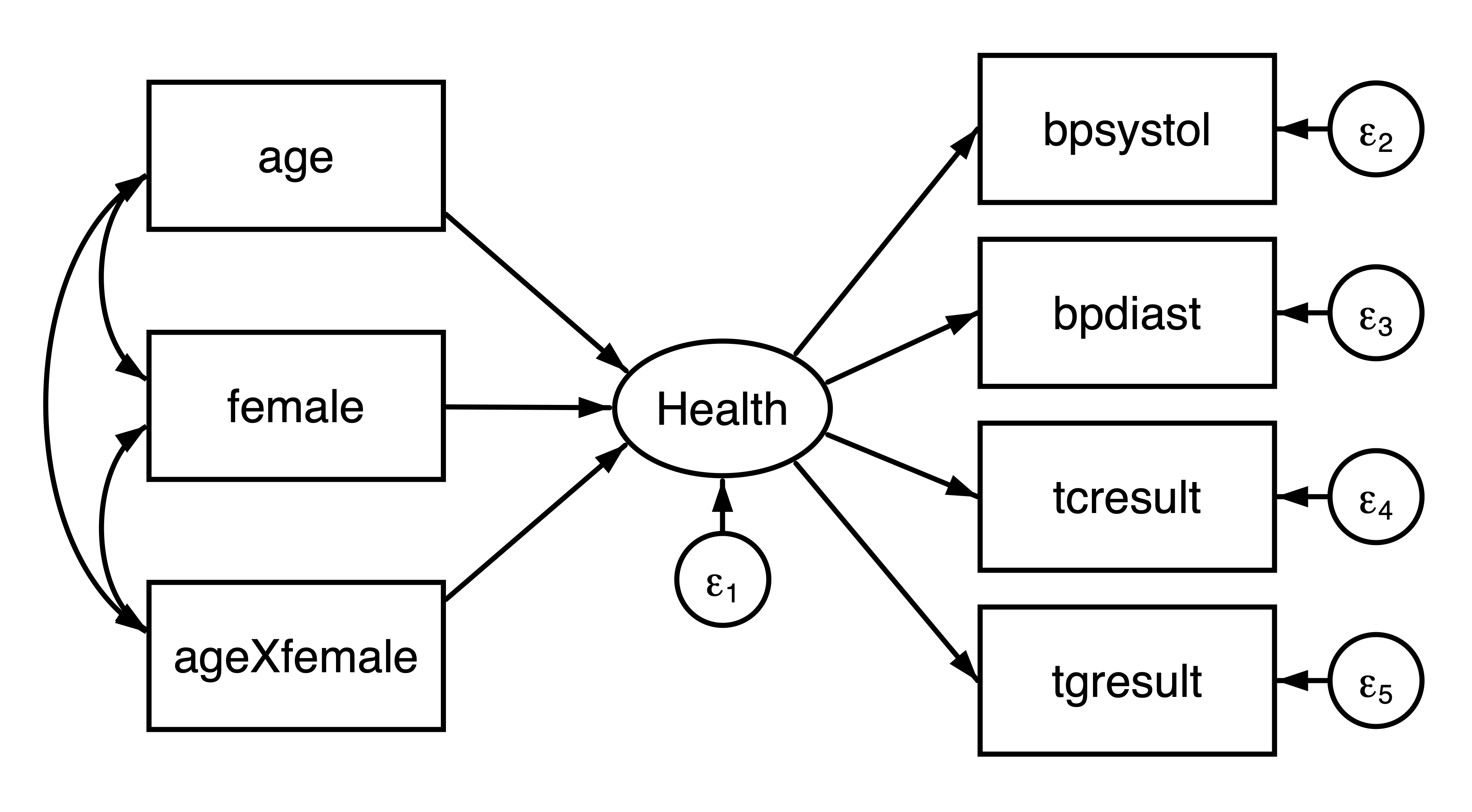
We’re planning a brand new examine to guage the interplay impact between age and intercourse on well being. We are able to use the NHANES dataset to acquire an affordable covariance matrix from which we will simulate new knowledge. We’ll outline well being as a latent variable measured by systolic blood stress (bpsystol), diastolic blood stress (bpdiast), serum ldl cholesterol (tcresult), and serum triglyercides (tgresult). Particularly, we wish to match the next mannequin:
Determine 1: Path diagram of the hypothesized mannequin
Step 1: Get hold of or derive a covariance matrix (and means, if relevant) that corresponds along with your hypothesized mannequin
We’re going to use the model-implied covariance matrix from becoming the above mannequin to the NHANES knowledge. First, we have to load the dataset, create the interplay variable, after which match our mannequin.
. webuse nhanes2

. gen ageXfemale = age*feminine

. sem (Well being -> bpsystol bpdiast tcresult tgresult)
>    (age feminine ageXfemale -> Well being), nolog
(5301 observations with lacking values excluded)

Endogenous variables
  Measurement: bpsystol bpdiast tcresult tgresult
  Latent:      Well being

Exogenous variables
  Noticed: age feminine ageXfemale

Structural equation mannequin                                Variety of obs = 5,050
Estimation technique: ml

Log chance = -140667.36

 ( 1)  [bpsystol]Well being = 1
------------------------------------------------------------------------------
             |                 OIM
             | Coefficient  std. err.      z    P>|z|     [95% conf. interval]
-------------+----------------------------------------------------------------
Structural   |
  Well being     |
         age |   .4371085   .0237304    18.42   0.000     .3905977    .4836193
      feminine |  -20.89331    1.67081   -12.50   0.000    -24.16804   -17.61859
  ageXfemale |   .3395419   .0328812    10.33   0.000     .2750961    .4039878
-------------+----------------------------------------------------------------
Measurement  |
  bpsystol   |
      Well being |          1  (constrained)
       _cons |   111.2516   1.207464    92.14   0.000      108.885    113.6182
  -----------+----------------------------------------------------------------
  bpdiast    |
      Well being |   .4404182   .0096514    45.63   0.000     .4215018    .4593346
       _cons |   72.88132   .5554644   131.21   0.000     71.79263    73.97001
  -----------+----------------------------------------------------------------
  tcresult   |
      Well being |   .6630559   .0373398    17.76   0.000     .5898712    .7362406
       _cons |   203.6104   1.217816   167.19   0.000     201.2235    205.9973
  -----------+----------------------------------------------------------------
  tgresult   |
      Well being |   1.122149   .0726778    15.44   0.000     .9797029    1.264594
       _cons |     123.03   2.275853    54.06   0.000     118.5694    127.4906
-------------+----------------------------------------------------------------
var(e.bpsy~l)|   67.62701   8.855679                      52.31863    87.41462
var(e.bpdi~t)|    80.1877   2.164596                      76.05544    84.54446
var(e.tcre~t)|   2083.505   42.75414                      2001.372     2169.01
var(e.tgre~t)|   8724.877   176.5499                      8385.617    9077.862
var(e.Well being)|   340.7899   11.08864                      319.7351    363.2312
------------------------------------------------------------------------------
LR take a look at of mannequin vs. saturated: chi2(11) = 1542.14        Prob > chi2 = 0.0000
Age, intercourse, and their interplay are all important predictors of Well being when carried out on 5,050 observations, however maybe you don’t have the assets to gather a pattern that enormous. How massive does your pattern must be to have 80% energy to detect an interplay between age and intercourse? To simulate knowledge for our energy evaluation, we will use the model-implied covariance reported with the fitted choice of the estat framework command. It will present a whole lot of output, so we’ll run it quietly and simply return what we’re inquisitive about: the fitted covariance and the fitted means. Our hypothesized SEM doesn’t embrace imply construction, so together with the means for our energy evaluation is pointless. Nonetheless, I’ll embrace them in all of the steps under in order that our code could be generalized to different sorts of SEMs.
. quietly estat framework, fitted

. matrix listing r(mu)

r(mu)[1,8]
      Noticed:   Noticed:   Noticed:   Noticed:     Latent:   Noticed:
      bpsystol     bpdiast    tcresult    tgresult      Well being         age
mu   129.84614   81.070693    215.9396   143.89584   18.594545   47.941386

      Noticed:   Noticed:
        feminine  ageXfemale
mu   .51663366   24.836832

. matrix listing r(Sigma)

symmetric r(Sigma)[8,8]
                       Noticed:   Noticed:   Noticed:   Noticed:
                       bpsystol     bpdiast    tcresult    tgresult
  Noticed:bpsystol   532.05333
   Noticed:bpdiast   204.54181   170.27163
  Noticed:tcresult   307.94061   135.62265   2287.6872
  Noticed:tgresult   521.15538   229.52632   345.55515   9309.6905
      Latent:Well being   464.42632   204.54181   307.94061   521.15538
       Noticed:age   179.49835    79.05434   119.01744   201.42383
    Noticed:feminine  -1.1112203  -.48940167  -.73680119  -1.2469544
Noticed:ageXfemale   64.672663   28.483019   42.881591   72.572343

                         Latent:   Noticed:   Noticed:   Noticed:
                         Well being         age      feminine  ageXfemale
      Latent:Well being   464.42632
       Noticed:age   179.49835   293.25241
    Noticed:feminine  -1.1112203   .06869774   .24972332
Noticed:ageXfemale   64.672663   155.35796   12.005288   729.20189
Discover that each our covariance and our means embrace noticed in addition to latent variables. We simply need the data that corresponds with the noticed variables, so we’ll must extract simply these parts of those matrices and save them to a brand new matrix. We are able to specify a spread of rows or columns utilizing .. between the beginning and ending row or column. When concatenating matrices collectively, commas are used to indicate a brand new column and backslashes () are used to indicate a brand new row.
. matrix mu = r(mu)[1,1..4],r(mu)[1,6..8]

. matrix Sigma = r(Sigma)[1..4,1..4],r(Sigma)[1..4,6..8]r(Sigma)[6..8,1..4],
>    r(Sigma)[6..8,6..8]

. matrix listing mu

mu[1,7]
      Noticed:   Noticed:   Noticed:   Noticed:   Noticed:   Noticed:
      bpsystol     bpdiast    tcresult    tgresult         age      feminine
mu   129.84614   81.070693    215.9396   143.89584   47.941386   .51663366

      Noticed:
    ageXfemale
mu   24.836832

. matrix listing Sigma

symmetric Sigma[7,7]
                       Noticed:   Noticed:   Noticed:   Noticed:
                       bpsystol     bpdiast    tcresult    tgresult
  Noticed:bpsystol   532.05333
   Noticed:bpdiast   204.54181   170.27163
  Noticed:tcresult   307.94061   135.62265   2287.6872
  Noticed:tgresult   521.15538   229.52632   345.55515   9309.6905
       Noticed:age   179.49835    79.05434   119.01744   201.42383
    Noticed:feminine  -1.1112203  -.48940167  -.73680119  -1.2469544
Noticed:ageXfemale   64.672663   28.483019   42.881591   72.572343

                       Noticed:   Noticed:   Noticed:
                            age      feminine  ageXfemale
       Noticed:age   293.25241
    Noticed:feminine   .06869774   .24972332
Noticed:ageXfemale   155.35796   12.005288   729.20189
Now we’ve got the covariance matrix and means we have to simulate our knowledge!
Step 2: Simulate a single dataset assuming the choice speculation, and match the mannequin
Subsequent we create a simulated dataset from our covariance matrix (and means) utilizing the drawnorm command. drawnorm simulates a variable or set of variables based mostly on pattern dimension, means, and covariance. Right here we’ll use a pattern dimension of 200.
. set seed 12345

. clear

. drawnorm bpsystol bpdiast tcresult tgresult age feminine ageXfemale,
>    n(200) means(mu) cov(Sigma)
(obs 200)
We are able to then use sem to suit the hypothesized mannequin to our simulated knowledge.
. sem (Well being -> bpsystol bpdiast tcresult tgresult)
>    (age feminine ageXfemale -> Well being), nolog

Endogenous variables
  Measurement: bpsystol bpdiast tcresult tgresult
  Latent:      Well being

Exogenous variables
  Noticed: age feminine ageXfemale

Structural equation mannequin                                  Variety of obs = 200
Estimation technique: ml

Log chance = -5599.7049

 ( 1)  [bpsystol]Well being = 1
------------------------------------------------------------------------------
             |                 OIM
             | Coefficient  std. err.      z    P>|z|     [95% conf. interval]
-------------+----------------------------------------------------------------
Structural   |
  Well being     |
         age |   .5016981   .1243038     4.04   0.000     .2580671    .7453291
      feminine |  -18.12394   8.529735    -2.12   0.034    -34.84191   -1.405964
  ageXfemale |   .2329537   .1611524     1.45   0.148    -.0828992    .5488066
-------------+----------------------------------------------------------------
Measurement  |
  bpsystol   |
      Well being |          1  (constrained)
       _cons |   111.2897   6.191827    17.97   0.000     99.15397    123.4255
  -----------+----------------------------------------------------------------
  bpdiast    |
      Well being |   .4507904   .0627156     7.19   0.000     .3278701    .5737107
       _cons |   73.00124   3.087596    23.64   0.000     66.94967    79.05282
  -----------+----------------------------------------------------------------
  tcresult   |
      Well being |   .5630107    .183409     3.07   0.002     .2035357    .9224857
       _cons |    207.841   6.011418    34.57   0.000     196.0588    219.6231
  -----------+----------------------------------------------------------------
  tgresult   |
      Well being |   .8698218   .3926678     2.22   0.027     .1002072    1.639436
       _cons |   126.6153    11.5315    10.98   0.000     104.0139    149.2166
-------------+----------------------------------------------------------------
var(e.bpsy~l)|   137.2281   53.00586                      64.36608    292.5695
var(e.bpdi~t)|   75.17043   12.98479                      53.58117    105.4586
var(e.tcre~t)|   2235.489   226.4431                      1832.949    2726.432
var(e.tgre~t)|   8917.533   902.1103                      7313.681     10873.1
var(e.Well being)|   303.1287   58.65825                      207.4491    442.9376
------------------------------------------------------------------------------
LR take a look at of mannequin vs. saturated: chi2(11) = 13.10          Prob > chi2 = 0.2866
To check the null speculation that the interplay time period equals zero, it is going to be simpler to conduct a Wald take a look at utilizing the take a look at command with sem than utilizing the lrtest command utilized in earlier posts. In our case, we may have extracted the p-value from the desk above, however this step could be tailored to check any speculation of curiosity.
. take a look at ageXfemale

 ( 1)  [Health]ageXfemale = 0

           chi2(  1) =    2.09
         Prob > chi2 =    0.1483
The p-value for our take a look at is 0.148, so we might not be capable to reject the null speculation that the interplay time period equals zero.
As mentioned within the earlier submit, the mannequin gained’t all the time converge when match to simulated datasets. Like combined, sem will retailer a worth of 1 to e(converged) if the mannequin converges and 0 in any other case. We’ll retailer the worth of e(converged) from the mannequin to a neighborhood macro named conv to maintain observe of the convergence of our fashions. We’ll additionally create a neighborhood variable, reject, that can maintain observe of whether or not the estimated interplay time period is important. The worth that’s saved in reject is decided by the conditional perform cond(). If the mannequin converged, then r(p)<0.05 might be evaluated. A price of 1 might be saved to reject if the Wald take a look at p-value, r(p), is lower than the alpha stage, right here specified as 0.05, and 0 in any other case. If the mannequin did not converge, then a lacking worth might be saved in reject.
. sem (Well being -> bpsystol bpdiast tcresult tgresult)
>    (age feminine ageXfemale -> Well being)

. native conv = e(converged)

. take a look at ageXfemale

. native reject = cond(`conv'==1, r(p)<.05, .)
Step 3: Write a program to create the datasets, match the fashions, and use simulate to check this system
Subsequent let’s write a program that creates datasets below the choice speculation, suits sem fashions, assessments the null speculation of curiosity, and makes use of simulate to run many iterations of this system. The first distinction between this program and the applications we’ve got written in earlier posts is that this program wants to just accept matrices as enter arguments. This is usually a little tough. What we have to do is specify the kind of enter as a string somewhat than a matrix. Then inside the program we are going to outline our matrices by their title, handed to this system as a string, that’s, mat C = `cov’. Lastly, we will use these matrices to simulate our knowledge with drawnorm, match our mannequin, and take a look at the null speculation. We’ve additionally added seize in entrance of the sem command to seize errors in case the mannequin doesn’t converge. The code block under comprises the syntax for this program, known as simsem.
seize program drop simsem
program simsem, rclass
    model 17
    // PARSE INPUT
    syntax, n(integer)      ///
        cov(string)         ///
        [ means(string)     ///
        alpha(real 0.05) ]
    // COMPUTE POWER
    quietly {
       drop _all
       mat C =`cov'
       mat m = `means'
       drawnorm bpsystol bpdiast tcresult tgresult age feminine ageXfemale, ///
            n(`n') means(m) cov(C)
       seize sem (Well being -> bpsystol bpdiast tcresult tgresult)         ///
            (age feminine ageXfemale -> Well being)
       native conv = e(converged)
       take a look at ageXfemale
      native reject = cond(`conv'==1, r(p)<`alpha', .)
    }
    // RETURN RESULTS
    return scalar reject = `reject'
    return scalar conv = `conv'
finish
We then use simulate to run simsem 10 occasions utilizing our covariance matrix and means for a pattern dimension of 200.
. simulate reject=r(reject) converged=r(conv), reps(10) seed(12345):
>    simsem, n(200) means(mu) cov(Sigma)

      Command:  simsem, n(200) means(mu) cov(Sigma)
       reject:  r(reject)
    converged:  r(conv)

Simulations (10)
----+--- 1 ---+--- 2 ---+--- 3 ---+--- 4 ---+--- 5
...x...x..
simulate saved two variables: reject and converged. The imply of converged is the convergence fee. The imply of reject is the ability to check the null speculation that the age by intercourse interplay time period equals zero.
. summarize reject

    Variable |        Obs        Imply    Std. dev.       Min        Max
-------------+---------------------------------------------------------
      reject |          8          .5    .5345225          0          1

. summarize converged

    Variable |        Obs        Imply    Std. dev.       Min        Max
-------------+---------------------------------------------------------
   converged |         10          .8     .421637          0          1
With a pattern dimension of 200, the mannequin converged in 8 of the ten repetitions (80%) and had an influence of fifty% to detect the interplay impact on Well being.
Step 4: Write a program known as power_cmd_simsem, which lets you run your simulations with energy
We may cease with our fast simulation if we had been solely in a particular set of assumptions. However it’s straightforward to put in writing an extra program named power_cmd_simsem that can enable us to make use of Stata’s energy command to create tables and graphs for a spread of pattern sizes. We simply want to incorporate the enter syntax as we did within the simsem command, simulate with the simsem command, and return the outcomes.
seize program drop power_cmd_simsem
program power_cmd_simsem, rclass
   model 17
   // PARSE INPUT
   syntax, n(integer)                       ///
          cov(string)                       ///
          [ alpha(real 0.05)                ///
          means(string)                     ///
          reps(integer 100) ]
   // COMPUTE POWER
   quietly simulate reject=r(reject) converged=r(conv), reps(`reps'):  ///
          simsem, n(`n') means(`means') cov(`cov') alpha(`alpha')
   // RETURN RESULTS
   return scalar N = `n'
   return scalar alpha = `alpha'
   quietly summarize reject
   return scalar energy = r(imply)
   quietly summarize converged
   return scalar conv_rate = r(imply)
finish
Step 5: (Non-compulsory) Write a program known as power_cmd_simsem_init so as to see convergence charges on your mannequin at totally different pattern sizes.
Convergence is commonly a problem in SEM simulation. In case your mannequin is having hassle converging at smaller pattern sizes, it could be helpful so as to add a convergence fee column to the ability output desk.
seize program drop power_cmd_simsem_init
program power_cmd_simsem_init, sclass
   model 17
   sreturn clear
   // ADD COLUMNS TO THE OUTPUT TABLE
   sreturn native pss_colnames "conv_rate"
finish
Utilizing energy simsem
Finally, we will use energy simsem to simulate energy and convergence fee for a spread of pattern sizes. The instance under simulates energy for pattern sizes starting from 200 to 500, utilizing 100 repetitions every.
. energy simsem, n(200(100)500) means(mu) cov(Sigma) reps(100)
>    desk(N conv_rate energy) graph
xxxxxxxxxxxxxxxxxxxxxxxxxxxxxx
Estimated energy
Two-sided take a look at

  +---------------------------+
  |       N conv_rate   energy |
  |---------------------------|
  |     200       .86      .5 |
  |     300       .92   .7283 |
  |     400       .93   .8602 |
  |     500       .97   .8866 |
  +---------------------------+
Determine 2: Estimated energy for a structural equation mannequin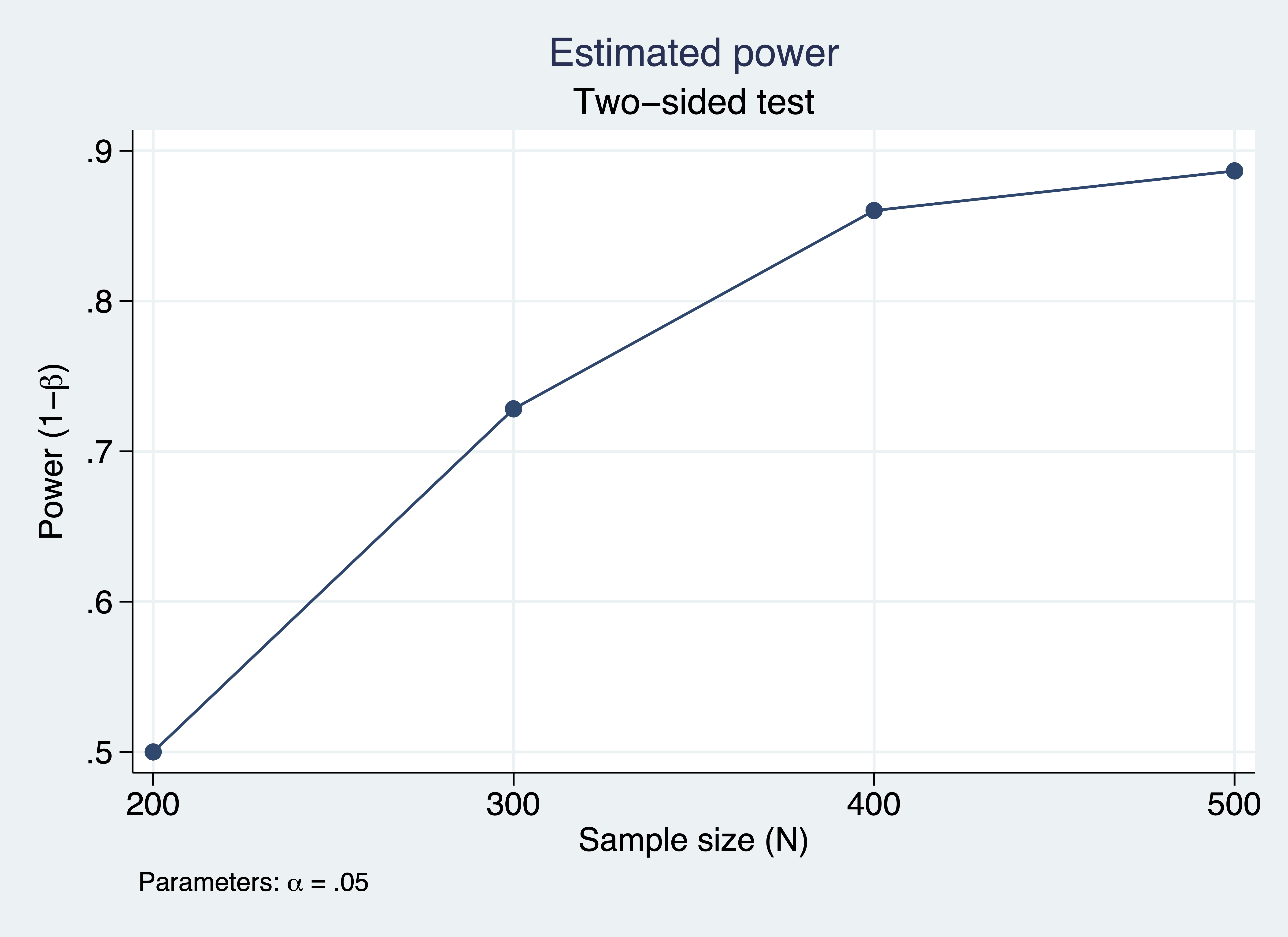
The desk and graph above point out that 80% energy is achieved round a pattern dimension of 350.
The process demonstrated right here can be utilized to carry out an influence evaluation on any SEM. You simply must outline your mannequin of curiosity and simulate knowledge based mostly on a covariance matrix. Together with the earlier posts on this collection, we’ve got now given examples of how you need to use Stata to carry out energy evaluation by simulation for quite a lot of fashions. You should use related strategies for nearly any energy evaluation it is advisable carry out.
Deriving covariances based mostly on SEM path coefficients utilizing the RAM technique
As mentioned originally of this submit, you need to use the RAM to instantly specify inhabitants parameters or use outcomes from a publication to acquire a covariance matrix. The RAM technique makes use of a set of matrices to symbolize the mannequin, which could be mixed utilizing matrix algebra to derive the corresponding covariance matrix. Three matrices are required: (mathbf{A}), (mathbf{S}), and (mathbf{F}). These comprise the trail coefficients, issue loadings, variances, and covariances of the mannequin you wish to simulate knowledge from. Moreover, a matrix of means, (mathbf{M}), is required if the SEM entails imply construction.
To display find out how to use mannequin outcomes to construct these matrices, we are going to use the outcomes from our knowledge evaluation on the NHANES datset. We’ll use the noxconditional choice within the sem command as a result of we’d like the estimated variances or covariances of the exogenous variables with a purpose to create our matrices.
. webuse nhanes2, clear

. gen ageXfemale = age*feminine

. sem (Well being -> bpsystol bpdiast tcresult tgresult)
>    (age feminine ageXfemale -> Well being), noxconditional nolog
(5301 observations with lacking values excluded)

Endogenous variables
  Measurement: bpsystol bpdiast tcresult tgresult
  Latent:      Well being

Exogenous variables
  Noticed: age feminine ageXfemale

Structural equation mannequin                                Variety of obs = 5,050
Estimation technique: ml

Log chance = -140667.36

 ( 1)  [bpsystol]Well being = 1
------------------------------------------------------------------------------
             |                 OIM
             | Coefficient  std. err.      z    P>|z|     [95% conf. interval]
-------------+----------------------------------------------------------------
Structural   |
  Well being     |
         age |   .4371086   .0237305    18.42   0.000     .3905977    .4836194
      feminine |  -20.89331    1.67081   -12.50   0.000    -24.16804   -17.61858
  ageXfemale |   .3395419   .0328812    10.33   0.000      .275096    .4039878
-------------+----------------------------------------------------------------
Measurement  |
  bpsystol   |
      Well being |          1  (constrained)
       _cons |   111.2516   1.207464    92.14   0.000      108.885    113.6182
  -----------+----------------------------------------------------------------
  bpdiast    |
      Well being |   .4404182   .0096514    45.63   0.000     .4215018    .4593346
       _cons |   72.88132   .5554643   131.21   0.000     71.79263    73.97001
  -----------+----------------------------------------------------------------
  tcresult   |
      Well being |   .6630558   .0373398    17.76   0.000     .5898711    .7362405
       _cons |   203.6104   1.217816   167.19   0.000     201.2235    205.9973
  -----------+----------------------------------------------------------------
  tgresult   |
      Well being |   1.122149   .0726778    15.44   0.000     .9797027    1.264594
       _cons |     123.03   2.275853    54.06   0.000     118.5694    127.4906
-------------+----------------------------------------------------------------
    imply(age)|   47.94139   .2409767   198.95   0.000     47.46908    48.41369
 imply(feminine)|   .5166337   .0070321    73.47   0.000      .502851    .5304163
imply(ageXf~e)|   24.83683   .3799953    65.36   0.000     24.09205    25.58161
-------------+----------------------------------------------------------------
var(e.bpsy~l)|   67.62698    8.85568                       52.3186    87.41459
var(e.bpdi~t)|    80.1877   2.164596                      76.05545    84.54447
var(e.tcre~t)|   2083.505   42.75414                      2001.372     2169.01
var(e.tgre~t)|   8724.877   176.5499                      8385.617    9077.862
var(e.Well being)|     340.79   11.08864                      319.7351    363.2313
     var(age)|   293.2524   5.835941                      282.0344    304.9166
  var(feminine)|   .2497233   .0049697                      .2401704    .2596562
var(ageXfe~e)|   729.2019   14.51166                      701.3071    758.2062
-------------+----------------------------------------------------------------
     cov(age,|
      feminine)|   .0686977   .1204256     0.57   0.568     -.167332    .3047275
     cov(age,|
  ageXfemale)|    155.358   6.864694    22.63   0.000     141.9034    168.8125
  cov(feminine,|
  ageXfemale)|   12.00529   .2541636    47.23   0.000     11.50714    12.50344
------------------------------------------------------------------------------
LR take a look at of mannequin vs. saturated: chi2(11) = 1542.14        Prob > chi2 = 0.0000
The primary matrix we are going to create is the (mathbf{A}) matrix. The (mathbf{A}) matrix is an uneven matrix that shops the single-headed path coefficients within the mannequin. The rows and columns of our matrix symbolize every of the noticed and latent variables. The cells symbolize paths from the column variable to the row variable. I’ll begin by making a matrix of 0s of the scale that I want utilizing J(r,c,z), an (r occasions c) matrix containing parts z. Then I’ll substitute blocks of cells with the paths from the mannequin into the (mathbf{A}) matrix. We solely must specify the higher left cell of the cells we’re substituting. Lastly, I’ll add row and column names to this matrix to make it simpler to interpret.
. matrix A = J(8,8,0)
. matrix A[1,8] = (1.00�.44�.661.12)
. matrix A[8,5] = (0.44,-20.89,0.34)
. matrix rownames A = bpsystol bpdiast tcresult tgresult age feminine
> ageXfemale Well being
. matrix colnames A = bpsystol bpdiast tcresult tgresult age feminine
> ageXfemale Well being
. matrix listing A
A[8,8]
bpsystol bpdiast tcresult tgresult age
bpsystol 0 0 0 0 0
bpdiast 0 0 0 0 0
tcresult 0 0 0 0 0
tgresult 0 0 0 0 0
age 0 0 0 0 0
feminine 0 0 0 0 0
ageXfemale 0 0 0 0 0
Well being 0 0 0 0 .44
feminine ageXfemale Well being
bpsystol 0 0 1
bpdiast 0 0 .44
tcresult 0 0 .66
tgresult 0 0 1.12
age 0 0 0
feminine 0 0 0
ageXfemale 0 0 0
Well being -20.89 .34 0
The (mathbf{S}) matrix is a symmetric matrix that shops double-headed path coefficients, variances, and covariances of our mannequin. I begin by making a diagnal matrix of all of the estimated variances from the mannequin, after which I add the covariances of the exogenous variables.
. matrix S = diag((67.63,80.19,2083.51,8724.88,0,0,0,340.79))
. matrix S[5,5] = (293.25,0.07,155.36�.07,0.25,12.01155.36,12.01,729.20)
. matrix rownames S = bpsystol bpdiast tcresult tgresult age feminine
> ageXfemale Well being
. matrix colnames S = bpsystol bpdiast tcresult tgresult age feminine
> ageXfemale Well being
. matrix listing S
symmetric S[8,8]
bpsystol bpdiast tcresult tgresult age
bpsystol 67.63
bpdiast 0 80.19
tcresult 0 0 2083.51
tgresult 0 0 0 8724.88
age 0 0 0 0 293.25
feminine 0 0 0 0 .07
ageXfemale 0 0 0 0 155.36
Well being 0 0 0 0 0
feminine ageXfemale Well being
feminine .25
ageXfemale 12.01 729.2
Well being 0 0 340.79
The (mathbf{F}) matrix is an oblong matrix to differentiate noticed and latent variables. The rows symbolize every noticed variable, and the columns symbolize every noticed and latent variable. Every row will get a `1′ within the cell of that variable’s corresponding column, making a diagonal submatrix. A diagonal matrix of 1s can be known as the id matrix. We are able to specify an id matrix with I(n) the place n is the variety of rows/columns. I add a column vector of 0s with J().
. matrix F = I(7),J(7,1,0)

. matrix rownames F = bpsystol bpdiast tcresult tgresult age feminine
>    ageXfemale

. matrix colnames F = bpsystol bpdiast tcresult tgresult age feminine
>    ageXfemale Well being

. matrix listing F

F[7,8]
              bpsystol     bpdiast    tcresult    tgresult         age
  bpsystol           1           0           0           0           0
   bpdiast           0           1           0           0           0
  tcresult           0           0           1           0           0
  tgresult           0           0           0           1           0
       age           0           0           0           0           1
    feminine           0           0           0           0           0
ageXfemale           0           0           0           0           0

                feminine  ageXfemale      Well being
  bpsystol           0           0           0
   bpdiast           0           0           0
  tcresult           0           0           0
  tgresult           0           0           0
       age           0           0           0
    feminine           1           0           0
ageXfemale           0           1           0
Lastly, in case your mannequin entails imply construction, an (mathbf{M}) matrix should even be created to acquire the model-implied means. That is only a column vector of estimated means or intercepts for the noticed and latent variables within the mannequin. Until explicitly estimated, you may assume all of the latent variable means are 0.
. matrix M = (111.2572.88203.61123.0347.94.5224.84�)
. matrix rownames M = bpsystol bpdiast tcresult tgresult age feminine
> ageXfemale Well being
. matrix listing M
M[8,1]
c1
bpsystol 111.25
bpdiast 72.88
tcresult 203.61
tgresult 123.03
age 47.94
feminine .52
ageXfemale 24.84
Well being 0
Now we will use matrix algebra to derive the model-implied means and covariance. The dimension of I() will must be modified based mostly on the variety of noticed and latent variables within the mannequin. Right here it’s 8 to incorporate the seven noticed variables and the one latent variable.
. *model-implied means
. matrix mu = F*inv(I(8)-A)*M

. matrix listing mu

mu[7,1]
                   c1
  bpsystol   129.9264
   bpdiast  81.097616
  tcresult  215.93642
  tgresult  143.94757
       age      47.94
    feminine        .52
ageXfemale      24.84

. *model-implied covariance
. matrix Sigma = F*inv(I(8)-A)*S*inv(I(8)-A)'*F'

. matrix listing Sigma

symmetric Sigma[7,7]
              bpsystol     bpdiast    tcresult    tgresult         age
  bpsystol   533.17918
   bpdiast   204.84164   170.32032
  tcresult   307.26246   135.19548   2286.3032
  tgresult   521.41508   229.42264   344.13395   9308.8649
       age    180.3901   79.371644   119.05747   202.03691      293.25
    feminine     -1.1083    -.487652    -.731478   -1.241296         .07
ageXfemale     65.3975     28.7749    43.16235     73.2452      155.36

                feminine  ageXfemale
    feminine         .25
ageXfemale       12.01       729.2
We see the covariance matrix implied by the mannequin with the equipped mannequin parameters.