
In a earlier submit I confirmed an instance through which the “textbook” confidence interval for a proportion performs poorly regardless of a reasonably large pattern measurement. My purpose in that submit was to persuade you that the oft-repeated recommendation regarding (n > 30) and the central restrict theorem is nugatory. Immediately I’d prefer to persuade you of one thing much more subversive: the textbook confidence interval for a proportion is completely horrible and it is best to by no means use it or educate it beneath any circumstances. Fortuitously there’s a easy repair. For a 95% interval, merely add 4 “faux” observations to your dataset, two successes and two failures, after which observe the textbook recipe for this “artificially augmented” dataset.
This submit attracts on two very approachable papers from across the flip of the millennium: Agresti & Coull (1998) and Brown, Cai, & DasGupta (2001). Extra theoretically-inclined readers may get pleasure from a companion paper to the latter reference: Brown, Cai, & DasGupta (2002).
That is what you discovered in your introductory statistics course: it’s the textbook interval I alluded to above. Let (X_1, …, X_n sim textual content{iid Bernoulli}(p)) and outline (widehat{p} = sum_{i=1}^n X_i/n). By the central restrict theorem
[
frac{widehat{p} – p}{sqrt{widehat{p}(1 – widehat{p})/n}} rightarrow_d N(0,1)
]
resulting in the so-called “Wald” 95% confidence interval for a inhabitants proportion:
[
widehat{p} pm 1.96 times sqrt{frac{widehat{p}(1- widehat{p})}{n}}.
]
Suppose we need to estimate the proportion of Trump voters in Berkeley California. We resolve perform a ballot of 25 randomly-sampled Berkeley residents and discover that none of them voted for Trump. Then (widehat{p} = 0) and the Wald confidence interval is
[
0 pm 1.96 times sqrt{0 times (1 – 0) / 25}
]
in different phrases ([0, 0]). Clearly that is absurd: until there are actually zero Trump voters in Berkeley, we will be sure that this interval doesn’t include the true inhabitants parameter. The same downside would emerge if we as an alternative tried to estimate the proportion of Biden voters within the Berkeley: if (widehat{p} = 1) then our confidence interval can be ([1,1]). This too is absurd. Extra broadly, the Wald confidence interval is extraordinarily poorly behaved in conditions the place (p) is near zero or one. You could have encountered a suggestion that (np(1-p)) ought to be at the very least 5 for the Wald interval to carry out nicely. There’s one thing to this recommendation, as we’ll see beneath, nevertheless it’s not enough. Extra to the purpose: we don’t know (p) in apply so there is no such thing as a technique to apply this rule!
Right here’s a fast and soiled repair that’s suprisingly efficient. Merely add 4 “faux” observations to the dataset: two zeros (failures) and two ones (successes). The 95% Agresti-Coull confidence interval is constructed in precisely the identical method as 95% Wald interval solely utilizing this “artificially augmented” dataset moderately than the unique one. In different phrases, if the pattern measurement is (n) and the pattern proportion is (widehat{p}), then Agresti-Coull interval is constructed from (widetilde{n} = n + 4) and
[
widetilde{p} equiv frac{n widehat{p} + 2}{n + 4} = frac{left(sum_{i=1}^n X_iright) + 0 + 0 + 1 + 1}{n + 4}
]
yielding
[
widetilde{p} pm 1.96 times sqrt{frac{widetilde{p}(1 – widetilde{p})}{widetilde{n}}}, quad widetilde{n} equiv n + 4, quad widetilde{p} equiv frac{nwidehat{p}+ 2}{n + 4}.
]
Be aware that this “add 4 faux observations” adjustment is restricted to the case of a 95% confidence interval. In a future submit, I’ll clarify the place the rule comes from and learn how to generalize it to different confidence ranges. For now, let’s ask ourselves a extra basic query: does this adjustment make sense? “Wait!” I can hear you object: “including faux observations introduces a bias!” Certainly it does. Since (widehat{p}) is an unbiased estimator of (p),
[
begin{aligned}
text{Bias}(widetilde{p}) &equiv mathbb{E}[widetilde{p} – p] = mathbb{E}left[ frac{n widehat{p} + 2}{n + 4}right] – p
&= frac{np + 2}{n+4} – p = (1 – 2p) left(frac{2}{n + 4}proper).
finish{aligned}
]
If (p = 1/2) this estimator is unbiased. In any other case, the addition of 4 faux observations pulls (widetilde{p}) away from (widehat{p}) and in the direction of (1/2): when (p>1/2) the estimator is downward-biased, and when (p < 1/2) it’s upward-biased. The smaller the pattern measurement, the bigger the bias.
Let’s do this out on our Trump/Berkeley instance. Including 4 faux observations provides a pattern proportion of
[
widetilde{p} = frac{n widehat{p} + 2}{n + 4} = frac{25 times 0 + 2}{25 + 4} = frac{2}{29} approx 0.07
]
within the augmented dataset and therefore a 95% confidence interval of roughly
[
0.07 pm 1.96 times sqrt{frac{0.07 times (1 – 0.07)}{29}} = [-0.02, 0.16].
]
After all a proportion can’t be adverse, so we’d report ([0, 0.16]). This looks as if a way more cheap abstract of our uncertainty than reporting an interval of ([0,0]), however does it actually work? Does including faux information actually enhance issues?
To reply the query raised on the finish of the final paragraph, let’s use R to calculate the protection chance of the Wald and Agresti-Coull intervals for a variety of values of the pattern measurement (n) and true inhabitants proportion (p). In different phrases, let’s see how usually these intervals truly include the true inhabitants parameter (p). If they’re bona fide 95% confidence intervals, this could happen with chance near 0.95. One technique to perform this train is through Monte Carlo simulation: repeatedly drawing randomly generated datasets and counting the proportion of our ensuing confidence intervals that include the true worth of (p). On this instance, nonetheless, it seems that there’s a fast and straightforward technique to calculate precise protection chances utilizing the R perform dbinom. For full particulars, see the R code appendix on the finish of the submit.
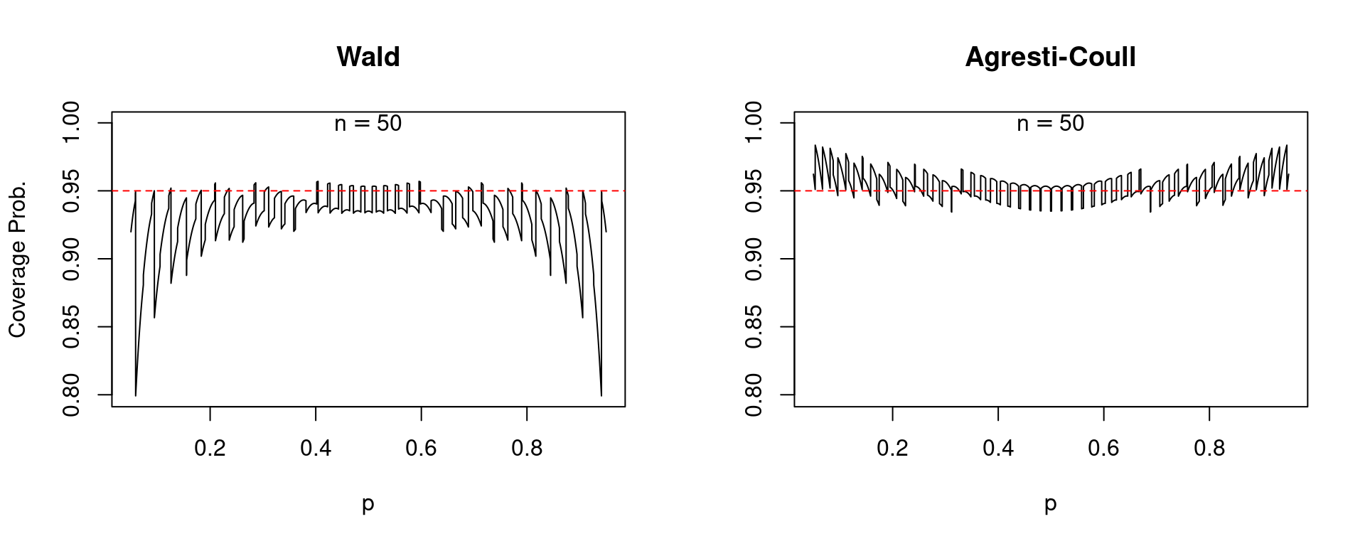
To start, let’s examine the 2 confidence intervals over a grid of values for the true inhabitants proportion (p) whereas holding the pattern measurement (n) mounted. When (n = 25) we get hold of the next:
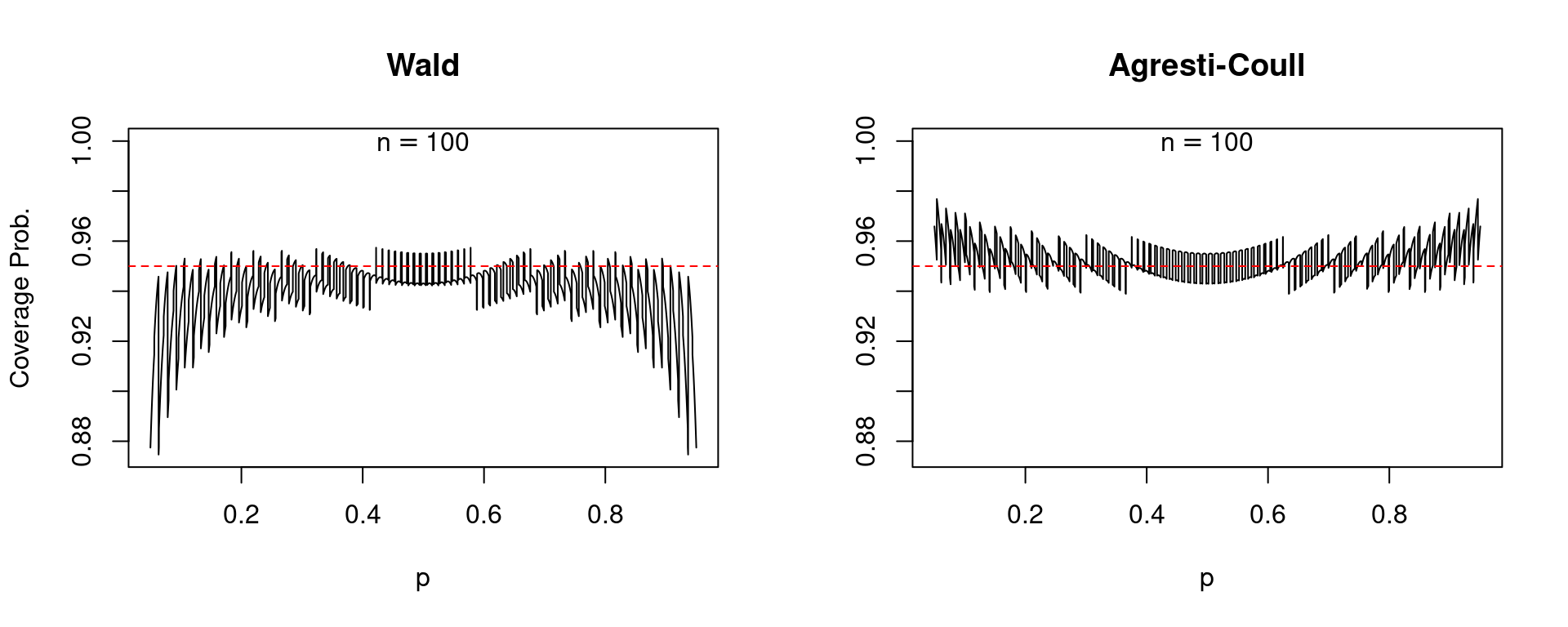
In every of those plots, together with those who observe, the stable black curve provides the protection chance whereas the dashed purple line passes via (0.95) on the vertical axis. A well-behaved confidence interval ought to produce a black curve that’s near the dashed purple line. To make a protracted story quick: the Agresti-Coull interval is kind of well-behaved whereas the Wald interval is a catastrophe. For values of (p) near zero or one, the Wald interval is extraordinarily erratic: its protection chance will be precisely 95% or far beneath relying on the exact worth of (p). Furthermore, the Wald interval systematically undercovers. There are only a few values of (p) for which its protection chance is 0.95 or greater and really many for which it’s beneath this stage. In stark distinction, the Agresti-Coull interval at worst undercovers by round 0.01 or 0.02. Basically its precise protection chance could be very near 95%, though it does generally tend to overcover for values of (p) which are near zero or one. It seems that there’s nothing particular about (n = 25). The identical primary story holds for bigger pattern sizes, for instance (n=50) and (n = 100).
So what can we make of the rule of thumb that the Wald interval will carry out nicely if (np(1-p)>5)? Certainly, values of (p) which are near zero or one current the most important issues for this confidence interval. However like many conventional statistical guidelines of thumb, this one leaves a lot to be desired. Suppose that (n = 1270) and (p = 0.005). On this case (np(1-p)) equals 6.3 however the protection chance of the Wald interval is an unsatisfying 0.875 in comparison with 0.958 for the Agresti-Coull interval.
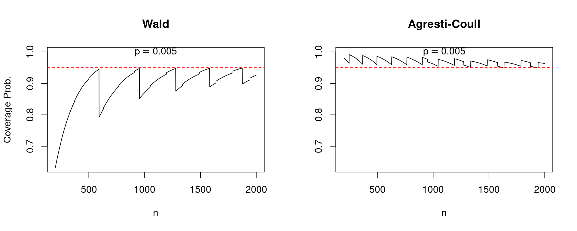
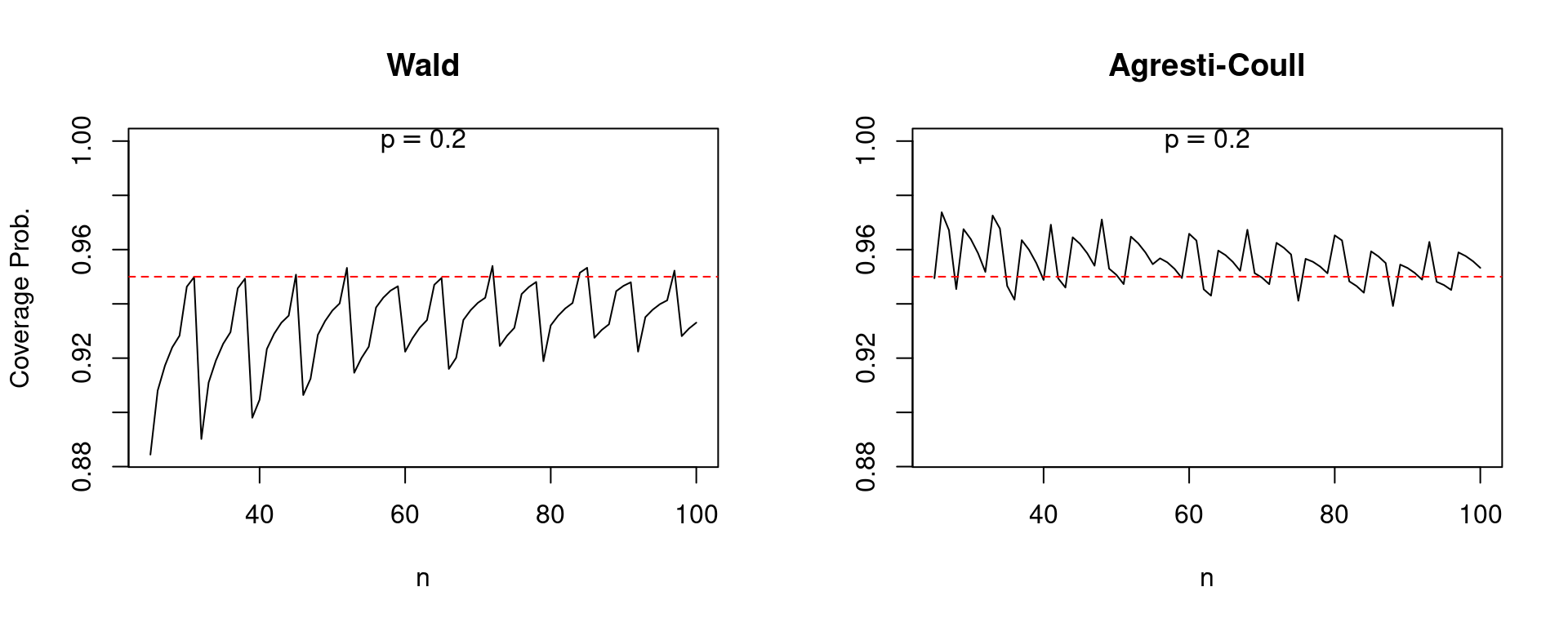
As a result of the central restrict theorem is an asymptotic consequence, one which holds as (n) approaches infinity, we would hope that at the very least the efficiency of the Wald interval improves because the pattern measurement grows. Alas, this isn’t all the time the case. The next plot compares the protection of Wald and Agresti-Coull confidence intervals for (p = 0.005) as (n) will increase from 200 to 2000. Be aware the pronounced “sawtooth” sample within the Wald confidence interval. It improves steadily because the pattern measurement grows solely to leap precipitously downward, earlier than starting a gentle upward climb adopted by one other soar. In distinction, the efficiency of the Agresti-Coull interval is pretty regular. Whereas a bit much less dramatic, the same qualitative sample holds for (p=0.2) as (n) will increase from 25 to 100.
Associates don’t let pals use the Wald interval for a proportion. Fortuitously there’s a easy various if you’re after a 95% confidence interval: add two successes and two failures to your dataset, then proceed as regular. I encourage you to make use of my R code to check out totally different values of (p) and (n), making your individual comparisons of the Wald and Agresti-Coull intervals. In a future submit, I’ll present you the place the Agresti-Coull interval comes from, why it really works so nicely, and learn how to generalize it to assemble 90%, 99% and certainly arbitrary ((1 – alpha) instances 100%) confidence intervals.
I wrote 4 R features to generate the plots proven above: get_Wald_coverage() and get_AC_coverage() calculate the protection chances of the Wald and Agresti-Coull confidence intervals, whereas plot_n_comparison() and plot_p_comparison() assemble the plots evaluating protection chances throughout totally different values of the pattern measurement (n) and true inhabitants proportion (p).
get_Wald_coverage <- perform(p, n) {
#-----------------------------------------------------------------------------
# Calculates the precise protection chance of a nominal 95% Wald confidence
# interval for a inhabitants proportion.
#-----------------------------------------------------------------------------
# p   true inhabitants proportion
# n   pattern measurement
#-----------------------------------------------------------------------------
  x <- 0:n
  p_hat <- x / n
  z <- qnorm(1 - 0.05 / 2)
  SE <- sqrt(p_hat * (1 - p_hat) / n)
  cowl <- (p >= p_hat - z * SE) & (p <= p_hat + z * SE)
  prob_cover <- dbinom(x, n, p)
  sum(cowl * prob_cover)
}

get_AC_coverage <- perform(p, n) {
#-----------------------------------------------------------------------------
# Calculates the precise protection chance of a nominal 95% Agresti-Coull
# confidence interval for a inhabitants proportion.
#-----------------------------------------------------------------------------
# p   true inhabitants proportion
# n   pattern measurement
#-----------------------------------------------------------------------------
  x <- 0:n
  p_tilde <- (x + 2) / (n + 4)
  n_tilde <- n + 4
  z <- qnorm(1 - 0.05 / 2)
  SE <- sqrt(p_tilde * (1 - p_tilde) / n_tilde)
  cowl <- (p >= p_tilde - z * SE) & (p <= p_tilde + z * SE)
  prob_cover <- dbinom(x, n, p)
  sum(cowl * prob_cover)
}

plot_n_comparison <- perform(n_seq, p) {
#-----------------------------------------------------------------------------
# Plots a comparability of protection chances for Wald and Agresti-Coull
# nominal 95% confidence intervals for a inhabitants proportion over a grid of
# values for the pattern measurement, holding the inhabitants proportion mounted.
#-----------------------------------------------------------------------------
# n_seq   vector of values for the pattern measurement
# p       true inhabitants proportion
#-----------------------------------------------------------------------------
# Instance:
#   my_p_seq <- seq(0.02, 0.98, 0.0001)
#   plot_p_comparison(my_p_seq, n = 25)
#-----------------------------------------------------------------------------
  wald <- sapply(n_seq, perform(n) get_Wald_coverage(p, n))
  AC <- sapply(n_seq, perform(n) get_AC_coverage(p, n))
  cover_min <- min(min(wald), min(AC))
  cover_max <- max(max(wald), max(AC))
  limits <- c(cover_min, 1)
  par(mfrow = c(1, 2))
  plot(n_seq, wald, sort = 'l', xlab = 'n', ylim = limits, fundamental = 'Wald',
       ylab = 'Protection Prob.')
  textual content(imply(n_seq), 1, labels = bquote(p == .(p)))
  abline(h = 0.95, lty = 2, col = 'purple')
  plot(n_seq, AC, sort = 'l', xlab = 'n', ylim = limits,
       fundamental = 'Agresti-Coull', ylab = '')
  textual content(imply(n_seq), 1, labels = bquote(p == .(p)))
  abline(h = 0.95, lty = 2, col = 'purple')
  par(mfrow = c(1, 1))
}

plot_p_comparison <- perform(p_seq, n) {
#-----------------------------------------------------------------------------
# Plots a comparability of protection chances for Wald and Agresti-Coull
# nominal 95% confidence intervals for a inhabitants proportion over a grid of
# values for the inhabitants proportion, holding pattern measurement mounted.
#-----------------------------------------------------------------------------
# p_seq   vector of values for the true inhabitants proportion
# n       pattern measurement
#-----------------------------------------------------------------------------
# Instance:
#   plot_n_comparison(n_seq = 25:100, p = 0.2)
#-----------------------------------------------------------------------------
  wald <- sapply(p_seq, perform(p) get_Wald_coverage(p, n))
  AC <- sapply(p_seq, perform(p) get_AC_coverage(p, n))
  cover_min <- min(min(wald), min(AC))
  limits <- c(cover_min, 1)
  par(mfrow = c(1, 2))
  plot(p_seq, wald, sort = 'l', xlab = 'p', ylim = limits, fundamental = 'Wald',
       ylab = 'Protection Prob.')
  textual content(0.5, 1, labels = bquote(n == .(n)))
  abline(h = 0.95, lty = 2, col = 'purple')
  plot(p_seq, AC, sort = 'l', xlab = 'p', ylim = limits,
       fundamental = 'Agresti-Coull', ylab = '')
  textual content(0.5, 1, labels = bquote(n == .(n)))
  abline(h = 0.95, lty = 2, col = 'purple')
  par(mfrow = c(1, 1))
}