Visualizing medical code hierarchy with treemaps

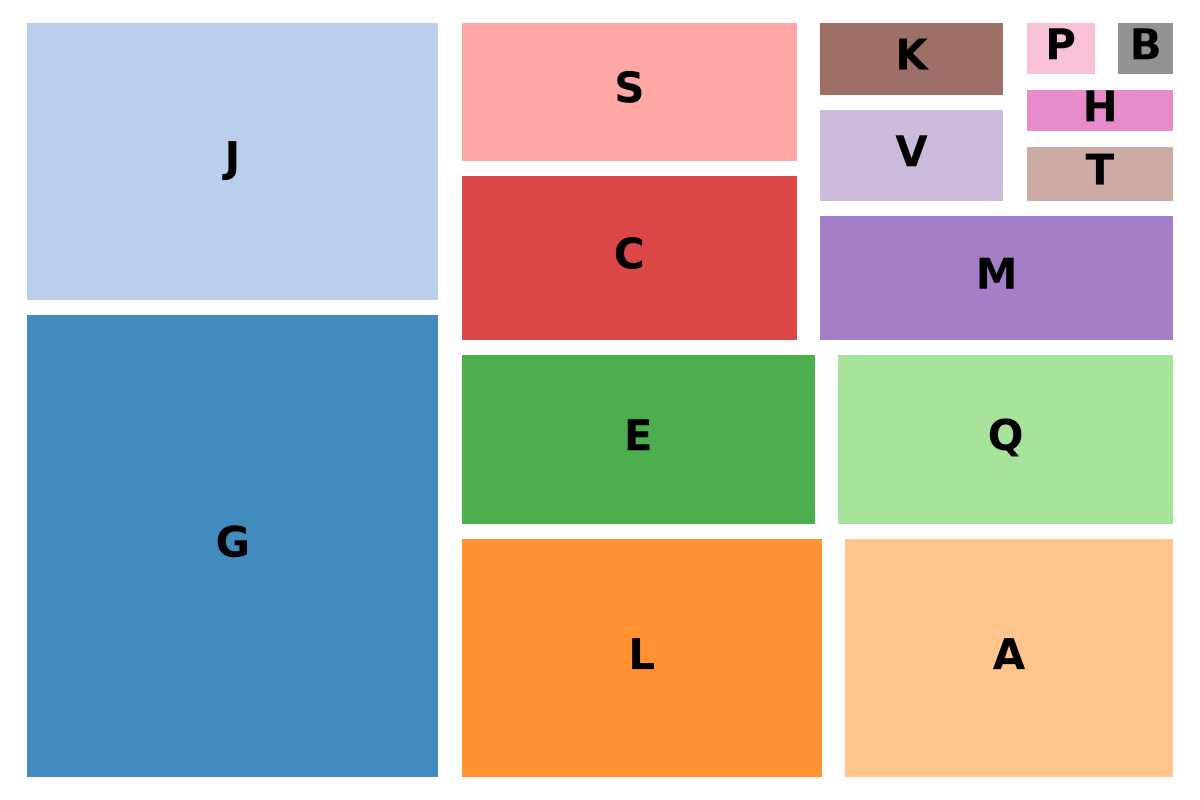
Fast observe as much as the earlier two posts on ICD-10 codes and HCPCS codes. This publish makes use of Python’s squarify library to create treemaps visualizing what number of codes start with every letter.

Right here’s the treemap for HCPCS codes.

And right here’s the treemap for ICD-10 codes.

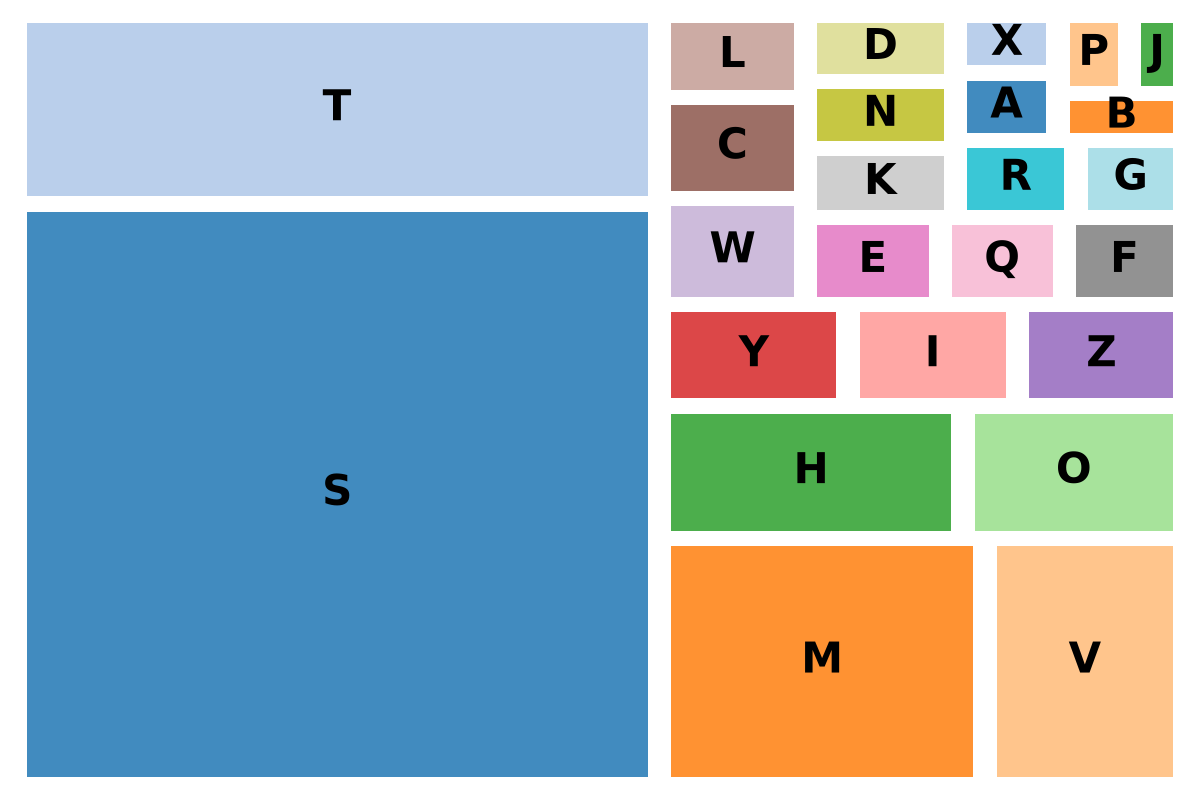
The sizes of the squares are proportional to the variety of codes starting with that letter. Notice that they don’t seem to be essentially proportional to how usually codes are used.

The HCPCS map omits R and U as a result of these are tiny relative to the remainder. The ICD-10 map omits U for a similar cause.

Right here’s the code that was used to create the HCPCS map.

import matplotlib.pyplot as plt
import squarify

# HCPCS
information = {
    "G": 2010,
    "J": 1232,
    "L": 940,
    "A": 862,
    "E": 671,
    "Q": 639,
    "C": 619,
    "S": 533,
    "M": 506,
    "V": 212,
    "Ok": 175,
    "T": 114,
    "H": 94,
    "P": 59,
    "B": 51,
  # "U": 5,
  # "R": 3,
}

labels = record(information.keys())
sizes = record(information.values())

# Labels are simply the letters (no counts)
display_labels = labels

# Coloration map — one distinct shade per field
colours = plt.cm.tab20.colours[: len(labels)]

fig, ax = plt.subplots(figsize=(12, 8))
squarify.plot(
    sizes=sizes,
    label=display_labels,
    shade=colours,
    alpha=0.85,
    ax=ax,
    text_kwargs={"fontsize": 30, "weight": "daring"},
    pad=True,
)
ax.axis("off")

plt.tight_layout()
plt.savefig("treemap.png", dpi=72)
plt.present()

The code to create the ICD-10 map differs solely in its information.

# ICD-10
information = {
    "S": 31052, 
    "T": 10090, 
    "M":  6665, 
    "V":  4086, 
    "H":  3330, 
    "O":  2437, 
    "Y":  1590, 
    "I":  1427, 
    "Z":  1411, 
    "W":  1290, 
    "C":  1226, 
    "L":  1000, 
    "E":   971, 
    "Q":   894, 
    "F":   871, 
    "Ok":   857, 
    "N":   836, 
    "D":   824, 
    "R":   773, 
    "G":   700, 
    "A":   573, 
    "X":   495, 
    "B":   495, 
    "P":   463, 
    "J":   360, 
  # "U":     3,
}