Reproducing a geometry theorem diagram

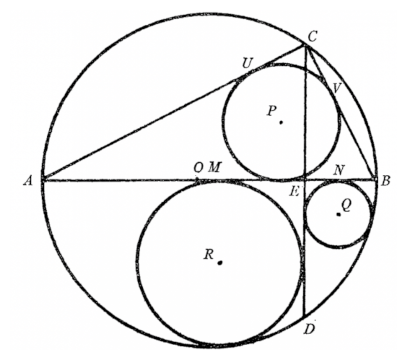
I ran throughout a geometry theorem with the next diagram.

The concept equivalent to the diagram is fascinating, however I discovered reproducing the diagram extra fascinating.

The phase AB is a diameter and the road CD is perpendicular to the diameter.

Assume the outer circle is a unit circle. I guessed C = (cos(1), sin(1)) and made the next diagram.

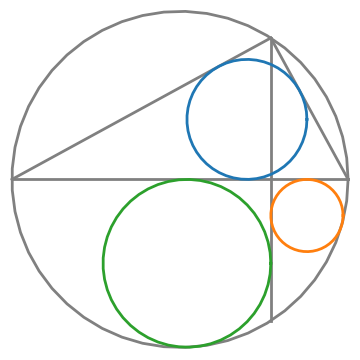
I guessed the worth of C by eyeballing it, however looking back this could have been a handy worth for the creator of the unique diagram to have chosen.

Drawing the blue circle inscribed within the triangle was simple utilizing the equations for the middle and radius from this put up. Drawing the opposite two circles, the inexperienced and orange circles, was more durable. They’re additionally inscribed circles, however not inscribed in a triangle. They’re inscribed in a three-sided determine with two perpendicular sides and a round arc.

The radius r of the inexperienced circle is the space from the middle of the circle to every of its tangent strains. Additionally, the space from the origin to the middle of the circle should be 1 − r. That is sufficient info to arrange a quadratic equation for r. The identical reasoning applies to the orange circle.

The unique diagram comes from [1] and the theory it illustrates says the diameter of the blue circle equals the sum of the radii of the inexperienced and orange circles.

Python code

In case you’re , right here’s the code that created the diagram.

#!/usr/bin/env -S uv run --script

# /// script
# dependencies = ["numpy", "matplotlib"]
# ///

import numpy as np
import matplotlib.pyplot as plt

def join(A, B, colour="grey"):
    plt.plot([A[0], B[0]], [A[1], B[1]], colour=colour, linewidth=2)

def circle(c, r, colour="grey"):
    t = np.linspace(0, 2*np.pi)
    plt.plot(c[0] + r*np.cos(t), c[1] + r*np.sin(t), colour=colour, linewidth=2)

def quadratic(a, b, c):
    det = b**2 - 4*a*c
    return ((-b - det**0.5)/(2*a), (-b + det**0.5)/(2*a))

A = np.array([-1, 0])
B = np.array([ 1, 0])
C = np.array([np.cos(1), np.sin(1)])
a = np.linalg.norm(B - C)
b = np.linalg.norm(A - C)
c = np.linalg.norm(B - A)
s = (a + b + c)/2

circle([0,0], 1)
join(A, B,)
join(A, C)
join(C, B)
join(C, C*np.array([1, -1]))

middle = (a*A + b*B + c*C)/(2*s)
radius = 0.5*a*b/s
circle(middle, radius, 'C0')

Ex = C[0]
roots = quadratic(1, 2 + 2*Ex, Ex**2 - 1)
r = roots[1] # Smaller root is negaive
print(roots)
middle = (r + Ex, -r)
circle(middle, r, 'C1')

roots = quadratic(1, 2 - 2*Ex, Ex**2 - 1)
r = roots[1] # Smaller root is negaive
middle = (Ex - r, -r)
circle(middle, r, 'C2')

plt.gca().set_aspect("equal")
plt.axis("off")
plt.present()

[1] Leon Bankoff. A Geometrical Coincidence. Arithmetic Journal, Vol. 37, No. 5 (Nov., 1964), p. 324.