

Motivation
In an period of large-scale experimentation and wealthy observational information, the one-size-fits-all paradigm is giving option to individualized decision-making. Whether or not concentrating on messages to voters, assigning medical remedies to sufferers, or recommending merchandise to shoppers, practitioners more and more search to tailor interventions based mostly on particular person traits. This shift hinges on understanding how remedy results fluctuate throughout people, not simply whether or not interventions work on common, however for whom they work greatest.
Why is the typical remedy impact not adequate?
Conventional causal inference focuses on the typical remedy impact (ATE), which might masks vital heterogeneity. A drug may present modest common advantages whereas delivering transformative outcomes for some sufferers and proving dangerous for others. The conditional common remedy impact (CATE) captures this variation by estimating remedy results conditional on particular person traits, enabling customized selections.
What are metalearners and why can we use them?
Estimating CATE is statistically difficult, notably with high-dimensional information. Conventional parametric approaches typically fail when relationships are nonlinear or when the variety of covariates approaches or exceeds the pattern dimension. To handle this, researchers have developed metalearners. They’re a versatile household of algorithms that cut back CATE estimation to a collection of supervised studying duties, leveraging highly effective machine studying fashions within the course of.
On this weblog submit, we offer an introduction to CATE and to 3 sorts of metalearners. We display the way to use the h2oml suite of instructions to estimate CATE utilizing every of the metalearners.
The flexibility to research detailed details about people and their habits inside massive datasets has sparked important curiosity from researchers and companies. This curiosity stems from a want to grasp how remedy results fluctuate amongst people or teams, transferring past merely understanding the ATE. On this context, the CATE perform is usually the first focus, outlined as
[
tau(mathbf{x}) = mathbb{E}{Y(1) – Y(0) mid mathbf{X} = mathbf{x}}
]
Right here (Y(1)) and (Y(0)) signify the potential outcomes if a topic is assigned to the remedy or management group, respectively. We situation on covariates (mathbf{X}). Usually, (mathbf{X}) needn’t include all noticed covariates. In apply, although, it typically does. With normal causal assumptions like overlap, positivity, and unconfoundedness, CATE is often recognized because the distinction between two regression capabilities,
[
tau(mathbf{x}) = mu_1(mathbf{x}) – mu_0(mathbf{x}) = mathbb{E}(Y mid mathbf{X} = mathbf{x}, T = 1) – mathbb{E}(Y mid mathbf{X} = mathbf{x}, T = 0) tag{1}label{eq:cate}
]
the place (T) represents the remedy variable. Be aware that individualized remedy results (ITE), (D_i = Y_i(1) – Y_i(0)), are generally conflated with CATE, however they aren’t the identical (Vegetabile 2021). ITEs and CATEs are solely equal if we think about all particular person traits (tilde{X}) related to their potential outcomes.
Early strategies for estimating (tau(mathbf{x})) typically assumed it was fixed or adopted a identified parametric type (Robins, Mark, and Newey 1992; Robins and Rotnitzky 1995). Nonetheless, current years have seen a surge of curiosity in additional versatile CATE estimators (van der Laan 2006; Robins et al. 2008; Künzel et al. 2019; Athey, Tibshirani, and Wager 2019; Nie and Wager 2020).
Beneath, we discover three strategies: the S-learner, T-learner, and X-learner. Our dialogue will largely observe the framework offered in Künzel et al. (2019). For a current overview, see Jacob (2021).
Dataset
For this submit, we use socialpressure.dta, borrowed from Gerber, Inexperienced, and Larimer (2008), the place the authors look at whether or not social stress can increase voter turnout in US elections. The voting habits information had been collected from Michigan households previous to the August 2006 main election by means of a large-scale mailing marketing campaign.
The authors randomly assigned registered voter households to obtain mailers. They used concentrating on standards based mostly on deal with info, together with a set of indices and voting habits, to unsolicited mail to households estimated to have a average likelihood of voting. The experiment included 4 remedy circumstances: civic responsibility, family, self and neighbors, and a management group.
We are going to focus solely on the management group (191,243 observations) and the self and neighbors remedy group (38,218 observations). The self and neighbors mailing included messages reminiscent of “DO YOUR CIVIC DUTY—VOTE” and an inventory of family and neighbors’ voting data. The mailer additionally knowledgeable the family that an up to date chart can be despatched after the elections. We are going to think about gender, age, voting in main elections in 2000, 2002, and 2004, and voting within the basic election in 2000 and 2002 as predictors.
We start by importing the dataset to Stata and making a variable, totalvote, that teams potential voters by their previous voting historical past. This variable takes values from 0 to five, the place 0 corresponds to people who didn’t vote in any of the 5 earlier elections and 5 corresponds to those that voted in all 5. Later, we use this variable to interpret CATE estimates by subgroup. For comfort, we generate a Stata body named social through the use of the body copy command.
. webuse socialpressure
(Social stress information)

. generate totalvote = g2000 + g2002 + p2000 + p2002 + p2004

. body copy default social
Subsequent we initialize an H2O cluster and put this dataset as an H2O body.
. h2o init
(output omitted)

. _h2oframe put, into(social)

Progress (%): 0 100
A metalearner is a high-level algorithm that decomposes the CATE estimation downside into a number of regression duties that may be tackled by your favourite machine studying fashions (base learners like random forest, gradient boosting machine [GBM], and their buddies).
There are three sorts of metalearners for CATE estimation: the S-learner, T-learner, and X-learner. The S-learner is the only of the thought of strategies. It matches a single mannequin, utilizing the predictors and the remedy as covariates. The T-learner improves upon this by becoming two separate fashions: one for the remedy group and one for the management group. The X-learner takes issues additional with a multistep process designed to leverage the complete dataset for CATE estimation. To maintain this submit from turning right into a theoretical marathon, we’ve tucked the deeper remedy of those strategies into an appendix. On this appendix, we demystify the logic behind these letters and clarify how every learner sequentially improves upon its predecessor. We strongly advocate that readers unfamiliar with these methods take a detour by means of the appendix earlier than leaping into the Stata implementation within the subsequent part.
It’s price noting that Stata’s cate command (see [CAUSAL] cate) implements the R-learner (Nie and Wager 2020) and generalized random forest (Athey, Tibshirani, and Wager 2019). The metalearners we talk about right here provide a complementary various to cate.
Implementation in Stata utilizing h2oml
S-learner
We begin by setting the H2O body social as our working body. Then, we create a worldwide macro, predictors, in Stata to include the predictor names and run gradient boosting binary classification utilizing the h2oml gbbinclass command. For illustration functions, we don’t implement hyperparameter tuning and pattern splitting. For particulars, see Jacob (2021). Nonetheless, in apply, all fashions used on this weblog submit ought to be tuned to acquire the best-performing mannequin. For particulars, see Mannequin choice in machine studying in [H2OML] Intro.
. _h2oframe change social

. world predictors gender g2000 g2002 p2000 p2002 p2004 remedy age

. h2oml gbbinclass voted $predictors, h2orseed(19)
(output omitted)
Subsequent, we create two copies of the H2O social body, social0 and social1, the place the predictor remedy is the same as 0 and 1, respectively. We use these frames to acquire predictions
(hat{mu}(mathbf{x},1)) and (hat{mu}(mathbf{x},0)) as in part A.1.
. _h2oframe copy social social1

. _h2oframe change social1

. _h2oframe substitute remedy = "Sure"

. _h2oframe copy social social0

. _h2oframe change social0

. _h2oframe substitute remedy = "No"
We use the educated GBM mannequin to foretell voting possibilities on these frames, storing them as yhat0_1 and yhat1_1, through the use of the h2omlpredict command with the body() and pr choices.
. h2omlpredict yhat0_0 yhat0_1, body(social0) pr

Progress (%): 0 100

. h2omlpredict yhat1_0 yhat1_1, body(social1) pr

Progress (%): 0 100
Then, we use the _h2oframe cbind command to affix these frames and enter the joined body into Stata through the use of the _h2oframe get command. Lastly, in Stata, we generate the variable catehat_S, as in eqref{eq:cateslearner} in appendix A.1, by subtracting the yhat0_1 prediction from the yhat1_1 prediction.
. _h2oframe cbind social1 social0, into(be a part of)

. _h2oframe get yhat1_1 yhat0_1 totalvote $predictors utilizing be a part of, clear

. generate catehat_S = yhat1_1 - yhat0_1
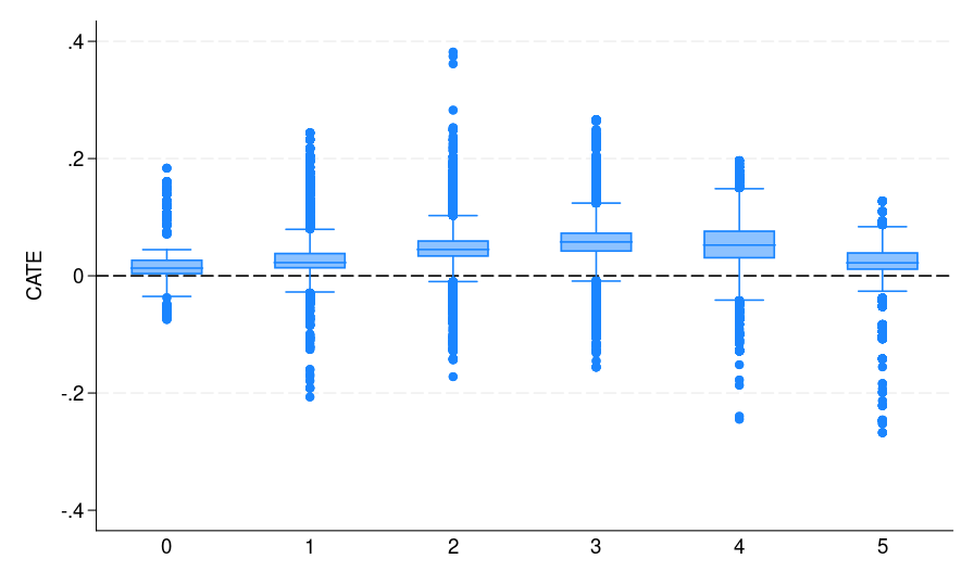
Be aware that catehat_S incorporates the CATE estimate from our S-learner. Determine 1(a) summarizes the outcomes, the place the potential voters are grouped by their voting historical past. It exhibits the distribution of CATE estimates for every of the subgroups. These outcomes may help marketing campaign organizers higher goal mailers sooner or later. As an illustration, if sources are restricted, specializing in potential voters who voted 3 times in the course of the previous 5 elections could also be handiest. This group not solely displays the best estimated ATE but additionally represents the biggest phase of potential voters, making it an excellent goal for maximizing affect.
|
|
|
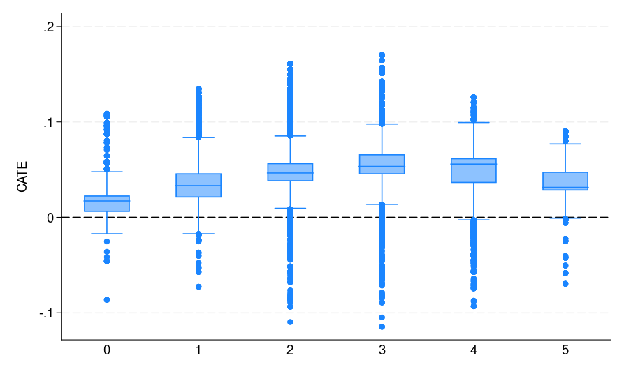
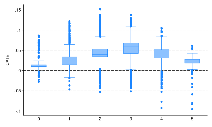
| (a) S-learner | (b) T-learner | (c) X-learner |
| Determine 1: The CATE estimate distribution for every bin, the place potential voters are grouped by the variety of elections they participated in | ||
Explainable machine studying for CATE
Machine studying fashions are sometimes handled as black bins that don’t clarify their predictions in a approach that practitioners can perceive. Explainable machine studying refers to strategies that depend on exterior fashions to make the selections and predictions of these fashions presentable and comprehensible to a human.
The dialogue on this part applies to all sorts of studying strategies mentioned on this weblog. For illustration, we present solely the S-learner. Having CATE estimates from the earlier sections, we are able to construct a surrogate mannequin, for instance, GBM, for CATE utilizing the predictors and use the out there explainable technique within the h2oml suite of instructions to elucidate CATE predictions. For out there, explainable instructions, see Interpretation and clarification in [H2OML] Intro.
To display, we are going to deal with exploring SHAP values and making a partial dependence plot. We begin by importing the present dataset in Stata as an H2O body. Then, to ensure that the issue variables have an accurate H2O sort enum, we use the _h2oframe issue command with the substitute choice. Then, we run gradient boosting regression for the estimated CATEs in catehat_S. As talked about above, we advise tuning this mannequin as effectively.
. _h2oframe put, into(social_cat) present
(output omitted)

. _h2oframe issue gender g2000 g2002 p2000 p2002 p2004 remedy, substitute

. h2oml gbregress catehat_S $predictors, h2orseed(19)
(output omitted)
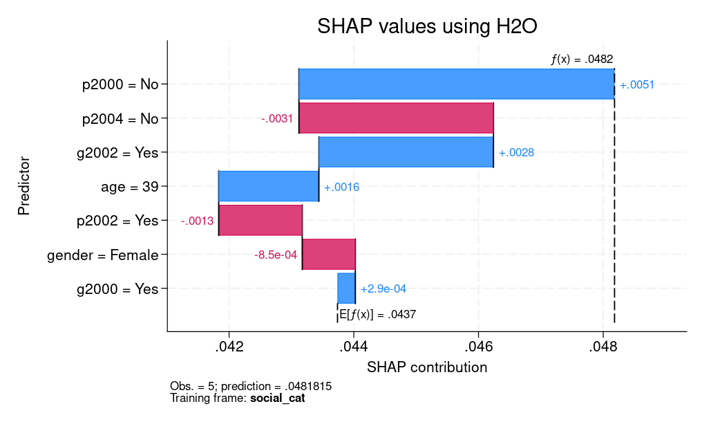
We graph the SHAP values and create a partial dependence plot (PDP) for explainability.
. h2omlgraph shapvalues, obs(5)

. h2omlgraph pdp age
(output omitted)
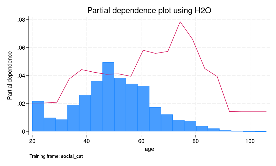
Determine 2 presents each SHAP values for a person prediction and a PDP for age. For SHAP values, we clarify the fifth commentary, which corresponds to a feminine who’s 39 years outdated. We are able to see that the age of 39 and voting within the 2002 basic elections however not voting within the 2000 main elections contribute positively to explaining the distinction between the person’s CATE prediction (0.0482) and the typical prediction of 0.0437. Nonetheless, not voting within the 2004 main elections had a detrimental contribution.
From the PDP, the purple line exhibits a rise in predicted CATE between ages 30 and 40, adopted by a small lower after which a rise from round age 60 to 80. One doable interpretation of the plateau and modest dip between 40 and 60 is that people in that age group could exhibit extra secure voting patterns which can be more durable to affect utilizing social stress mailers.
We may equally discover SHAP values for different people and PDP plots for different predictors.
|
|
| (a) SHAP values | (b) PDP |
| Determine 2: Explainable machine studying for CATE: (a) SHAP values (b) PDP | |
Subsequent we display the way to implement the T-learner. We start by splitting the dataset into two H2O frames: one for management observations (social0) and one other for handled observations (social1). These frames might be used to suit separate fashions for predicting outcomes within the handled and management teams, as described in appendix A.2.
. // T-learner step 1: Break up information by remedy group
. body change social

. _h2oframe put if remedy == 0, into(social0) substitute // management group
(output omitted)

. _h2oframe put if remedy == 1, into(social1) substitute // handled group
(output omitted)
Subsequent we use the h2oml gbbinclass command to coach a gradient boosting binary classification mannequin on the management group information, with voted as the result. The predictor names are specified utilizing the predictors macro, outlined earlier. We retailer this mannequin utilizing h2omlest retailer so we are able to later reload it for predictions within the subsequent part.
. // T-learner step 2: Practice a GBM mannequin for the management response perform
. _h2oframe change social0

. h2oml gbbinclass voted $predictors, h2orseed(19) // GBM mannequin: predict voting for T=group (management)
(output omitted)

. h2omlest retailer M0                                // Retailer mannequin as MO

. h2omlpredict yhat0_0 yhat0_1, body(social) pr   // Predict yhat0_1 = Pr(Y=1|X,T=0) based mostly on mannequin MO for full pattern

Progress (%): 0 100
After coaching the management mannequin, we change to the handled group body and practice one other GBM mannequin, once more utilizing voted as the result. This mannequin is saved individually and represents our estimate of the remedy response perform.
. // T-learner step 3: Practice a GBM mannequin for the remedy response perform
. _h2oframe change social1

. h2oml gbbinclass voted $predictors, h2orseed(19) // GBM mannequin: predict voting for T=1 group (handled)
(output omitted)

. h2omlest retailer M1                                // Retailer mannequin as M1

. h2omlpredict yhat1_0 yhat1_1, body(social) pr   // Predict yhat1_1 = Pr(Y=1|X,T=1) based mostly on mannequin M1 for full pattern

Progress (%): 0 100
As soon as each fashions are educated, we use them to generate counterfactual predictions yhat0_1 and yhat1_1 for all people within the full dataset. These predictions correspond to (hat{mu}_0(mathbf{x})) and (hat{mu}_1(mathbf{x})) in eqref{eq:catetlearner} in appendix A.2. We then compute their distinction in Stata and retailer it as catehat_T, which corresponds to the T-learner estimate of CATE (hat{tau}_T(mathbf{x})). Final, we plot the distribution of the CATE estimates by voting historical past [figure 1(b)] to evaluate how remedy results fluctuate throughout subgroups. It may be seen that each S- and T-learners (additionally the X-learner) present related CATE estimates.
. // T-learner step 4: Estimate CATE and visualize
. body change default

. _h2oframe get yhat1_1 yhat0_1 totalvote utilizing social, clear

. generate double catehat_T = yhat1_1 - yhat0_1  // CATE = handled prediction - management prediction

. graph field catehat_T, over(totalvote) yline(0) ytitle("CATE")
The X-learner begins through the use of the beforehand educated end result fashions, M0 and M1 from the T-learner, to generate counterfactual predictions. Particularly, we use the management group mannequin to foretell what handled people would have finished underneath management [(hat{mu}_0(X_i^1))] and the handled group mannequin to foretell what management people would have finished underneath remedy [(hat{mu}_1(X_i^0))].
. // X-learner step 1: Predict counterfactual outcomes for handled items
. h2omlest restore M0                              // Restore (load) management mannequin

. h2omlpredict yhat0_0 yhat0_1, body(social1) pr  // Predict yhat0_1 = Pr(Y=1|X,T=0) for handled items

Progress (%): 0 100

. // X-learner step 2: Predict counterfactual outcomes for management items
. h2omlest restore M1                              // Restore (load) handled mannequin
(outcomes M1 are lively now)

. h2omlpredict yhat1_0 yhat1_1, body(social0) pr // Predict yhat1_1 = Pr(Y=1|X,T=1) for management items

Progress (%): 0 100
Subsequent we compute imputed remedy results by subtracting these counterfactual predictions from noticed outcomes. For handled people, that is (tilde{D}_i^1 = Y^1_i – hat{mu}_0(X^1_i)), and for management people, it’s (tilde{D}_i^0 = hat{mu}_1(X^0_i) – Y^0_i). These imputed results function pseudooutcomes within the second stage of the X-learner. We then match regression fashions utilizing h2oml gbregress to foretell these pseudooutcomes (tilde{D}_i^1) and (tilde{D}_i^0) utilizing the unique covariates. These correspond to (hat{tau}_1(mathbf{x})) and (hat{tau}_0(mathbf{x})) in eqref{eq:catexlearner} in appendix A.3, that are the estimated CATE capabilities derived from the handled and management teams, respectively.
. // X-learner step 3: Impute remedy results for handled items
. _h2oframe change social1

. _h2oframe tonumeric voted, substitute           // Guarantee `voted' is numeric

. _h2oframe generate D1 = voted - yhat0_1      // Imputed impact = Y - counterfactual

. h2oml gbregress D1 $predictors, h2orseed(19) // Mannequin-imputed remedy results
(output omitted)

. h2omlpredict cate1, body(social)            // Predict cate1(x) = E(D1|X=x) on full pattern

. // X-learner step 4: Impute remedy results for management items
. _h2oframe change social0

. _h2oframe tonumeric voted, substitute

. _h2oframe generate D0 = yhat1_1 - voted      // Imputed impact = counterfactual - Y

. h2oml gbregress D0 $predictors, h2orseed(19)
(output omitted)

. h2omlpredict cate0, body(social)            // Predict cate0(x) = E(D0|X=x) on full pattern
Lastly, we mix these two CATE estimates saved in cate1 and cate0 utilizing a weighted common. In keeping with Künzel et al. (2019), we use a hard and fast weight (g(x)=0.5) for simplicity, though in apply this may be set to the estimated propensity rating (hat{e}(mathbf{x})).
. // X-learner step 5: Mix CATE estimates from each teams
. _h2oframe get cate0 cate1 totalvote utilizing social, clear

. native gx = 0.5                                                // Mix with weight (0.5 right here, might be e(x))

. generate double catehat_X = `gx' * cate0 + (1 - `gx') * cate1 // Closing CATE estimate

. graph field catehat_X, over(totalvote) yline(0) ytitle("CATE")
The distribution of the CATE estimates by voting historical past is displayed in determine 1(c).
As might be seen from determine 1, all S-, T-, and X-learners present related CATE estimates. This result’s anticipated given the very massive pattern dimension and small variety of predictors. Thus, it’s informative to debate when to undertake which learner. Following Künzel et al. (2019), we advise utilizing the S-learner when the researcher suspects that the remedy impact is easy or zero. If the remedy impact is strongly heterogeneous and the response end result distribution varies between remedy and management teams, then the T-learner may carry out effectively. Utilizing numerous simulation settings, Künzel et al. (2019) present that the X-learner successfully adapts to those completely different settings and performs effectively even when the remedy and management teams are imbalanced.
A metalearner is a high-level algorithm that decomposes the CATE estimation downside into a number of regression duties solvable by machine studying fashions (base learners like random forest, GBM, and so on.).
Let ( Y^0 ) and ( Y^1 ) denote the noticed outcomes for the management and remedy teams, respectively. As an illustration, ( Y^1_i ) is the result of the ( i )th unit within the remedy group. Covariates are denoted by ( mathbf{X}^0 ) and ( mathbf{X}^1 ), the place ( mathbf{X}^0 ) corresponds to the covariates of management items and ( mathbf{X}^1 ) to these of handled items; ( mathbf{X}^1_i ) refers back to the covariate vector for the ( i )th handled unit. The remedy project indicator is denoted by ( T in {0, 1} ), with ( T = 1 ) indicating remedy and ( T = 0 ) indicating management.
Regression fashions are represented utilizing the notation ( M_k(Y sim mathbf{X}) ), which denotes a generic studying algorithm, presumably distinct throughout fashions, that estimates the conditional expectation ( mathbb{E}(Y mid mathbf{X} = mathbf{x}) ) for given inputs. These fashions might be any machine studying estimator, together with versatile black-box learners. The primary estimand of curiosity is the CATE eqref{eq:cate}. That is the amount all metalearners are designed to estimate.
From eqref{eq:cate}, essentially the most easy factor to do is to simply implement a machine studying mannequin for the conditional expectation (E(Y|mathbf{X}, T)). The S-learner, the place the “S” stands for single, matches a single mannequin, utilizing each ( mathbf{X} ) and ( T ) as covariates:
[
mu(mathbf{x}, t) = mathbb{E}(Y mid mathbf{X} = mathbf{x}, T = t) quadtext{ which is estimated using }quad M{Y sim (mathbf{X}, T)}
]
The CATE estimator is given by
[
hat{tau}_S(mathbf{x}) = hat{mu}(mathbf{x},1) – hat{mu}(mathbf{x}, 0) tag{2}label{eq:cateslearner}
]
In apply, the remedy (T) is usually one-dimensional, whereas (mathbf{X}) might be high-dimensional. Trying on the CATE estimator in eqref{eq:cateslearner}, discover that the one enter to (hat{mu}) that modifications between the 2 phrases is (T). Consequently, if the machine studying mannequin used for estimation largely ignores (T) and primarily focuses on (mathbf{X}), the ensuing CATE may incorrectly be zero. The T-learner, mentioned subsequent, makes an attempt to handle this subject.
The query we are attempting to reply is, How can we ensure that the mannequin (hat{mu}) doesn’t ignore (T)? Properly, we are able to obtain this by coaching two completely different fashions for the remedy and management response capabilities (mu_1(mathbf{x})) and (mu_0(mathbf{x})), respectively. The T-learner, the place the “T” stands for 2, matches two separate fashions for the remedy and management teams:
start{align}
mu_1(mathbf{x}) &= mathbb{E}{Y(1) mid mathbf{X} = mathbf{x}, T = 1}, quad textual content{estimated by way of }quad M_1(Y^1 sim mathbf{X}^1)
mu_0(mathbf{x}) &= mathbb{E}{Y(0) mid mathbf{X} = mathbf{x}, T = 0}, quad textual content{estimated by way of }quad M_2(Y^0 sim mathbf{X}^0)
finish{align}
Then the CATE estimator is given by
[
hat{tau}_T(mathbf{x}) = hat{mu}_1(mathbf{x}) – hat{mu}_0(mathbf{x}) tag{3}label{eq:catetlearner}
]
To make sure (T) isn’t neglected, we practice two separate statistical fashions. First, we divide our information: ((Y^1,mathbf{X}^1)) consists of observations the place (T= 1), and ((Y^0,mathbf{X}^0)) of observations the place (T= 0). Then, we practice (M_1(Y^1 sim mathbf{X}^1)) to foretell (Y) for the (T=1) group and (M_2(Y^0 sim mathbf{X}^0)) to foretell (Y) for the group (T= 0).
Whereas the T-learner helps overcome the constraints of the S-learner, it introduces a brand new downside: it doesn’t make the most of all out there information when estimating (M_1) and (M_2). The X-learner, which we introduce subsequent, addresses this by making certain the complete dataset is used effectively for CATE estimation.
We first current the steps, then demystify their motivation. The X-learner proceeds in 4 steps:
- Match the result fashions:
[
hat{mu}_0(x) text{ using } M_1(Y^0 sim mathbf{X}^0) ; text{and }hat{mu}_1(x) text{ using } M_2(Y^1 sim mathbf{X}^1)
] - Compute imputed remedy results:
[
tilde{D}_i^1 = Y^1_i – hat{mu}_0(X^1_i), quad tilde{D}_i^0 = hat{mu}_1(X^0_i) – Y^0_i
] - Match the fashions to estimate:
start{align}
tau_1(mathbf{x}) &= mathbb{E}(tilde{D}^1 mid mathbf{X} = mathbf{x}), quad textual content{estimated by way of } quad M_3(tilde{D}^1 sim mathbf{X}^1)
tau_0(mathbf{x}) &= mathbb{E}(tilde{D}^0 mid mathbf{X} = mathbf{x}), quad textual content{estimated by way of } quad M_4(tilde{D}^0 sim mathbf{X}^0)
finish{align} - Mix estimates (hat{tau}_0(mathbf{x}) ) and (hat{tau}_1(mathbf{x}) ) to acquire the specified CATE estimator:
[
hat{tau}_X(mathbf{x}) = g(mathbf{x}) hat{tau}_0(mathbf{x}) + {1 – g(mathbf{x})} hat{tau}_1(mathbf{x}) tag{4}label{eq:catexlearner}
]
the place ( g(mathbf{x}) in [0,1] ) is a weight perform whose aim is to reduce the variance of (tau(mathbf{x})). An estimator of the propensity rating ( e(mathbf{x}) = mathbb{P}(T=1 mid mathbf{X}=mathbf{x}) ) is one doable alternative for (g(mathbf{x})).
As might be seen, step one of the X-learner is strictly the identical because the T-learner. Separate regression fashions are match to the remedy and management group information. The following two steps type the ingenuity of the strategy, as a result of that is the place all information from each fashions are utilized and the place the “X” (cross-estimation) in X-learner derives its that means. In step 2, (tilde{D}_i^1) and (tilde{D}_i^0) are the ITE estimates for the remedy and management teams, respectively. (tilde{D}_i^1) makes use of the remedy group outcomes and the imputed counterfactual obtained from (hat{mu}_0) in step 1. Analogously, (tilde{D}_i^0) is computed utilizing the management group outcomes and the imputed counterfactual estimated from (hat{mu}_1). This latter step ensures that the ITE estimates for every group make the most of information from each the remedy and management teams. Nonetheless, every of the estimates (tilde{D}_i^1) and (tilde{D}_i^0) makes use of solely a single commentary from its corresponding group. To handle this, the X-learner matches two completely different regression fashions in step 3, leading to two estimates: (hat{tau}_1(mathbf{x})), which intends to successfully estimate (E(Y^1|mathbf{X} = mathbf{x})), and (hat{tau}_0(mathbf{x})), which intends to estimate (E(Y^0|mathbf{X} = mathbf{x})). Lastly, step 4 combines these two estimates right into a single CATE estimate. Relying on the dataset, the selection of the load perform (g(mathbf{x})) could fluctuate. If the sizes of the remedy and management teams differ considerably, one may select (g(mathbf{x})=0) or (g(mathbf{x})=1) to prioritize one group’s estimate. In our evaluation, we use (g(x) = 0.5) to equally weight the estimates from each teams.
References
Athey, S., J. Tibshirani, and S. Wager. 2019. Generalized random forests. Annals of Statistics 47: 1148–1178. https://doi.org/10.1214/18-AOS1709.
Gerber, A., D. P. Inexperienced, and C. W. Larimer. 2008. Social stress and voter turnout: Proof from a large-scale discipline experiment. American Political Science Evaluate 102: 33–48. https://doi.org/10.1017/S000305540808009X.
Jacob, D. 2021. CATE meets ML: Conditional common remedy impact and machine studying. Dialogue Papers 2021-005, Humboldt-Universität of Berlin, Worldwide Analysis Coaching Group 1792. Excessive-Dimensional Nonstationary Time Collection.
Künzel, S. R., J. S. Sekhon, P. J. Bickel, and B. Yu. 2019. Metalearners for estimating heterogeneous remedy results utilizing machine studying. Proceedings of the Nationwide Academy of Sciences 116: 4156–4165. https://doi.org/10.1073/pnas.1804597116.
Nie, X., and S. Wager. 2020. Quasi-oracle estimation of heterogeneous remedy results. Biometrika 108: 299–319. https://doi.org/10.1093/biomet/asaa076.
Robins, J., L. Li, E. Tchetgen, and A. van der Vaart. 2008. Larger order affect capabilities and minimax estimation of nonlinear functionals. Institute of Mathematical Statistics Collections 2: 335–421. https://doi.org/10.1214/193940307000000527.
Robins, J. M., S. D. Mark, and W. Ok. Newey. 1992. Estimating publicity results by the expectation of publicity conditional on confounders. Biometrics 48: 479–495.
Robins, J. M., and A. Rotnitzky. 1995. Semiparametric effectivity in multivariate regression fashions with lacking information. Journal of the American Statistical Affiliation 90 122–129. https://doi.org/10.2307/2291135.
van der Laan, M. J. 2006. Statistical inference for variable significance. Worldwide Journal of Biostatistics Artwork. 2. https://doi.org/10.2202/1557-4679.1008.
Vegetabile, B. G. 2021. On the excellence between “conditional common remedy results” (CATE) and “particular person remedy results” (ITE) underneath ignorability assumptions. arXiv:2108.04939 [stat.ME]. https://doi.org/10.48550/arXiv.2108.04939.