


# Introduction
Most of you employ SQL window features, however you are solely scratching the floor — a ROW_NUMBER() right here, a SUM() OVER() there. The window features’ actual potential is revealed if you apply them to tougher issues. I’ll stroll you thru 4 patterns that present window features at their most helpful.
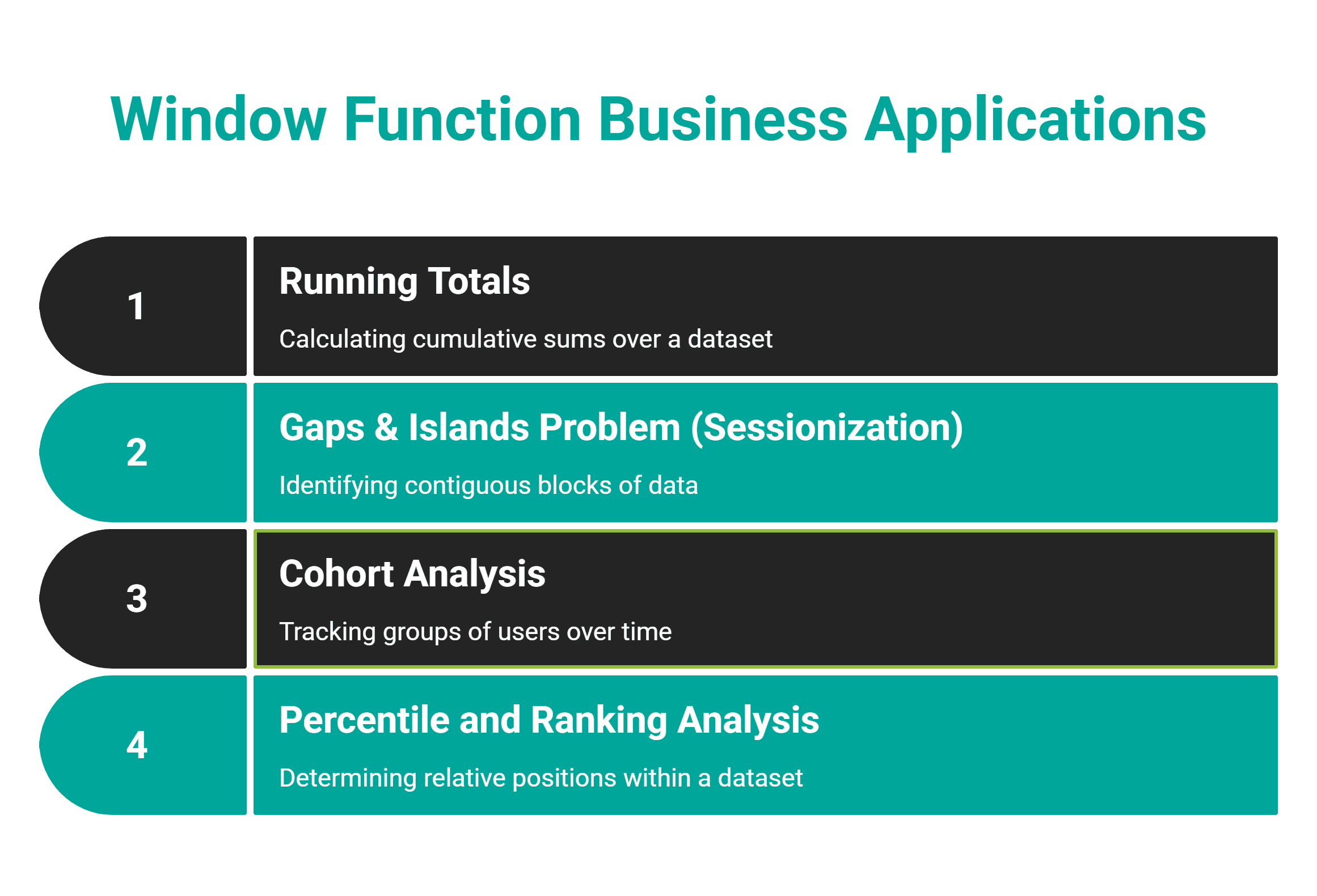
The examples are all actual interview questions you possibly can apply on StrataScratch.
# Operating Totals
Calculating operating totals is without doubt one of the most typical enterprise makes use of of window features. The finance individuals completely adore it! It’s used to trace cumulative month-to-month income, which then simply strikes into calculating the place you are at in comparison with the annual income goal.
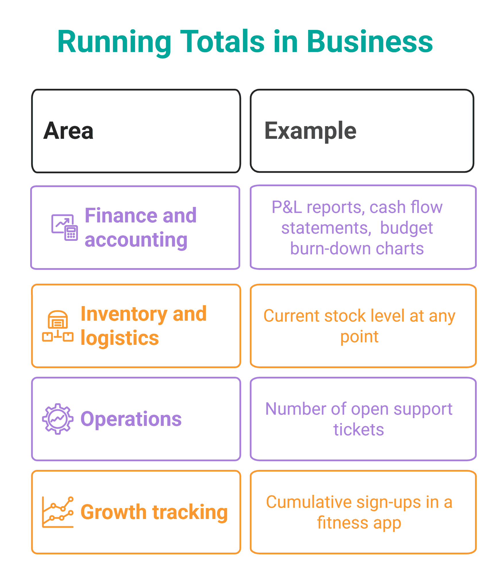
What makes this a window perform downside is that, usually, you need to embody each the per-period worth and the accumulating complete in the identical output. You may’t use GROUP BY with SUM(), as a result of that collapses particular person rows. So, the plain answer is utilizing a window perform, i.e., SUM() OVER().
// Instance: Calculating Income Over Time
This Amazon query initially asks you to calculate the 3-month rolling common. Nevertheless, we’ll disregard that and calculate the cumulative income for every month.
Knowledge: Here is the amazon_purchases desk preview.
| user_id | created_at | purchase_amt |
|---|---|---|
| 10 | 2020-01-01 | 3742 |
| 11 | 2020-01-04 | 1290 |
| 12 | 2020-01-07 | 4249 |
| … | … | … |
| 109 | 2020-10-24 | 1749 |
Code: The internal question turns dates into YYYY-MM format utilizing TO_CHAR() and aggregates month-to-month income, filtering out returns with WHERE purchase_amt > 0.
The outer question applies the window perform over these month-to-month totals we calculated. I do not specify an express body clause (deliberately) in OVER(), so the window perform defaults to RANGE BETWEEN UNBOUNDED PRECEDING AND CURRENT ROW. Which means the window is all rows previous the present row, i.e., the month. In different phrases, the cumulative sum is: all earlier months + the present month. Not surprisingly, that is a textbook definition of a cumulative sum.
SELECT t.month,
       t.monthly_revenue,
       SUM(t.monthly_revenue) OVER(ORDER BY t.month) AS cumulative_revenue
FROM (
    SELECT TO_CHAR(created_at::DATE, 'YYYY-MM') AS month,
        SUM(purchase_amt) AS monthly_revenue
    FROM amazon_purchases
    WHERE purchase_amt > 0
    GROUP BY TO_CHAR(created_at::date, 'YYYY-MM')
    ORDER BY TO_CHAR(created_at::date, 'YYYY-MM')
) t
ORDER BY t.month ASC;
Output:
| month | monthly_revenue | cumulative_revenue |
|---|---|---|
| 2020-01 | 26292 | 26292 |
| 2020-02 | 20695 | 46987 |
| 2020-03 | 29620 | 76607 |
| … | … | … |
| 2020-10 | 15310 | 239869 |
# Gaps and Islands (Sessionization)
This sample, too, includes sequential knowledge, identical to operating totals, nevertheless it employs totally different window features.
An island is a run of rows with the identical situation, e.g., consecutive day by day logins. A hole is the area between islands.
Probably the most frequent real-world functions of this sample is sessionization — grouping a uncooked occasion stream into classes. A session is usually outlined as a sequence of occasions from the identical consumer the place no hole between consecutive occasions exceeds some timeout (half-hour is the net analytics commonplace).
Sessionization is often utilized in product and knowledge engineering. It’s used anyplace you’ll want to group uncooked occasion streams into significant items of exercise.
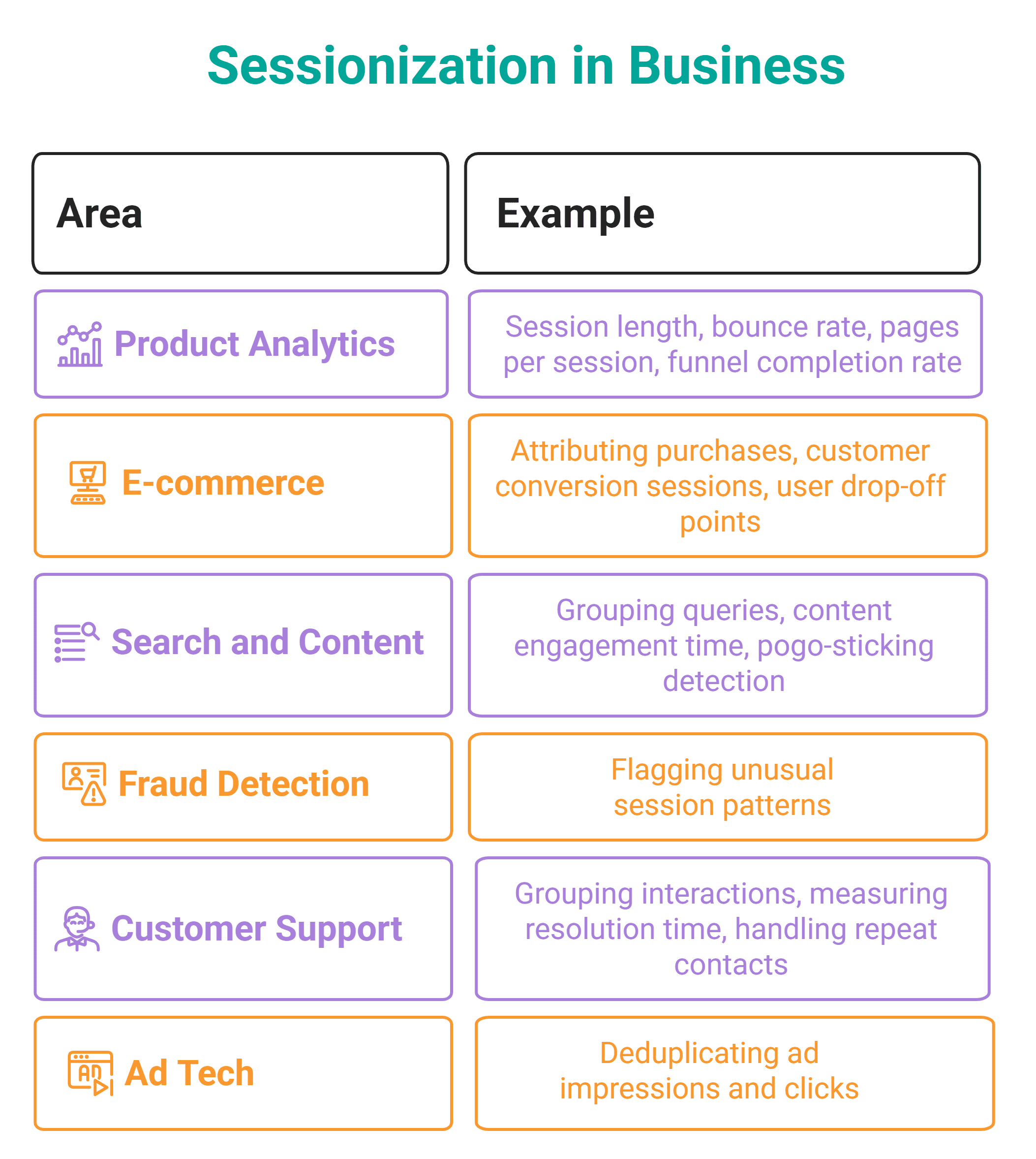
The basic detection in SQL consists of two steps:
LAG()orLEAD()— to check every row to the one earlier than or after it, and flag the place a brand new streak begins.SUM(flag) OVER (PARTITION BY consumer ORDER BY date)— to build up flags right into a streak ID, because it stays flat inside a streak and increments at each boundary.
// Instance: Discovering Person Streaks
The query from LinkedIn and Meta interviews asks you to search out the highest three customers with the longest platform go to streak till August 10, 2022. You need to output all customers with the highest three longest streaks, if there may be a couple of consumer per streak size.
Knowledge: The desk is user_streaks.
| user_id | date_visited |
|---|---|
| u001 | 2022-08-01 |
| u001 | 2022-08-01 |
| u004 | 2022-08-01 |
| … | … |
| u005 | 2022-08-11 |
Code: The question is lengthy, nevertheless it’s neatly structured into CTEs, so it is simple to comply with.
unique_visits: Removes duplicate go to information and caps the information at August 10, 2022.streak_flags: Makes use ofLAG()to get the earlier go to date per consumer and flags the row as0(a streak continuation if the hole is 1 day) or1(a brand new streak begin for every other hole).streak_ids: Converts flags into streak group IDs utilizing a cumulativeSUM().streak_lengths: Counts days per streak.longest_per_user: Retains solely every consumer’s longest streak.ranked_lengths: Ranks distinct streak lengths.top_lengths: Finds the highest 3 streak-length values.
The ultimate SELECT ties all the things collectively: it reveals all customers with the highest three streaks and their respective streak lengths in days.
WITH unique_visits AS (
    SELECT DISTINCT user_id, date_visited
    FROM   user_streaks
    WHERE  date_visited <= DATE '2022-08-10'),
streak_flags AS (
    SELECT *,
           CASE
               WHEN date_visited
                     - LAG(date_visited) OVER (PARTITION BY user_id ORDER BY date_visited) = 1
               THEN 0
               ELSE 1
           END AS new_streak
    FROM   unique_visits),
streak_ids AS (
    SELECT *,
           SUM(new_streak) OVER (PARTITION BY user_id ORDER BY date_visited) AS streak_id
    FROM   streak_flags),
streak_lengths AS (
    SELECT user_id,
           streak_id,
           COUNT(*) AS streak_length
    FROM   streak_ids
    GROUP  BY user_id, streak_id),
longest_per_user AS (
    SELECT user_id,
           MAX(streak_length) AS streak_length
    FROM   streak_lengths
    GROUP  BY user_id),
ranked_lengths AS (
    SELECT DISTINCT
           streak_length,
           DENSE_RANK() OVER (ORDER BY streak_length DESC) AS len_rank
    FROM   longest_per_user),
top_lengths AS (
    SELECT streak_length
    FROM   ranked_lengths
    WHERE  len_rank <= 3)
SELECT u.user_id,
       u.streak_length
FROM   longest_per_user u
JOIN   top_lengths       t USING (streak_length)
ORDER  BY u.streak_length DESC, u.user_id;
Output:
| user_id | streak_length |
|---|---|
| u004 | 10 |
| u005 | 10 |
| u003 | 5 |
| u001 | 4 |
| u006 | 4 |
# Cohort Evaluation
A cohort is a bunch of customers who share a beginning occasion, for instance, a primary buy, first login, or first subscription date. Analyzing cohorts is the basis of retention reporting, because it solutions the query of what number of customers got here again after the beginning occasion.
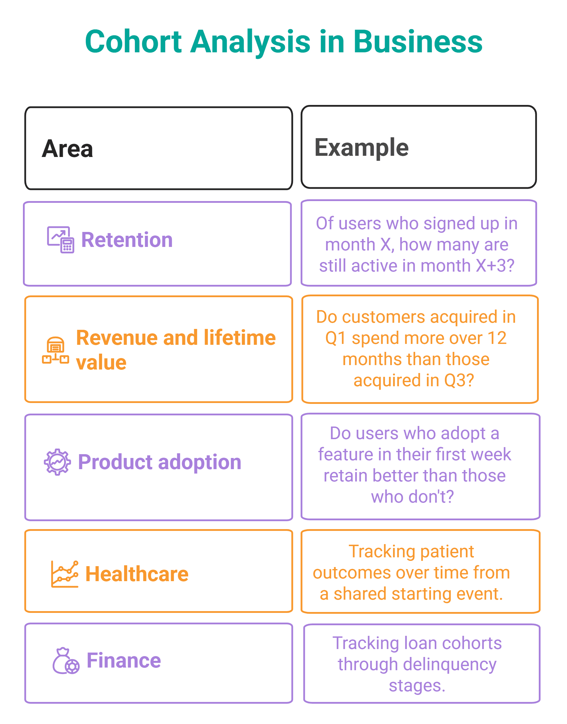
The important thing factor in cohort evaluation is discovering the cohort anchor within the consumer’s exercise historical past so to measure all subsequent exercise in opposition to it.
Doing that in SQL boils down to a few most important window perform approaches:
MIN(event_time) OVER (PARTITION BY user_id)— the commonest sample when the anchor is a date.FIRST_VALUE(attribute) OVER (PARTITION BY user_id ORDER BY event_time)— used if you want the anchor worth itself, e.g., the primary service provider or first product class.ROW_NUMBER() OVER (PARTITION BY user_id ORDER BY event_time) = 1— used if you wish to isolate the primary occasion as a separate row and be part of it again to the total historical past slightly than broadcasting it throughout all rows.
// Instance: Counting First-Time Orders
Here is a DoorDash query. It requires you to calculate the variety of orders and first-time orders (from a buyer’s perspective) every service provider has had. You also needs to exclude retailers that haven’t acquired any orders.
Knowledge: The primary desk is known as order_details.
| id | customer_id | merchant_id | order_timestamp | n_items | total_amount_earned |
|---|---|---|---|---|---|
| 8 | 1049 | 6 | 2022-01-14 01:00:28 | 5 | 16.3 |
| 7 | 1049 | 5 | 2022-01-14 11:50:29 | 4 | 2.16 |
| 22 | 1049 | 1 | 2022-01-14 22:46:54 | 8 | 2.63 |
| … | … | … | … | … | … |
| 39 | 1060 | 1 | 2022-01-16 22:27:30 | 11 | 15.41 |
The second desk is merchant_details.
| id | identify | class | zipcode |
|---|---|---|---|
| 1 | Treehouse Pizza | american | 92507 |
| 2 | Thai Lion | asian | 90017 |
| 3 | Meal Raven | quick meals | 95204 |
| … | … | … | … |
| 7 | Style Of Gyros | mediterranean | 94789 |
Code: The primary CTE is the place the cohort logic occurs. I take advantage of the FIRST_VALUE() window perform to connect the service provider from every buyer’s earliest order to each row of their order historical past. The result’s a desk the place each order carries the label of which service provider that buyer began with.
Within the second CTE, I be part of the labels again to the total order historical past utilizing a LEFT JOIN to make sure that retailers who acquired orders however had been by no means anybody’s first service provider nonetheless seem within the end result. We use COUNT() and DISTINCT to depend solely the shoppers for whom that service provider was their first — that is your cohort measurement. With one other COUNT(), you get the entire variety of orders. DISTINCT is required right here, too, as a result of the LEFT JOIN with first_order can produce duplicate order rows — since first_order retains one row per order (not per buyer), a single order in order_details can match a number of rows in first_order for a similar buyer, inflating the depend with out it.
Within the closing SELECT, we be part of the number_of_customers CTE with merchant_details to usher in the service provider names.
WITH first_order AS  (
SELECT customer_id,
       FIRST_VALUE(merchant_id) OVER(PARTITION BY customer_id ORDER BY order_timestamp) AS first_merchant
FROM order_details),
number_of_customers AS  (
SELECT merchant_id,
       COUNT(DISTINCT f.customer_id) AS first_time_orders,
       COUNT(DISTINCT id) AS total_number_of_orders
FROM order_details d
LEFT JOIN first_order f ON d.merchant_id = f.first_merchant
GROUP BY 1)
SELECT identify,
       total_number_of_orders,
       first_time_orders
FROM number_of_customers
JOIN merchant_details ON number_of_customers.merchant_id = merchant_details.id;
Output:
| identify | total_number_of_orders | first_time_orders |
|---|---|---|
| Treehouse Pizza | 8 | 1 |
| Thai Lion | 14 | 7 |
| Meal Raven | 12 | 0 |
| Burger A1 | 4 | 0 |
| Sushi Bay | 7 | 3 |
| Tacos You | 7 | 1 |
# Percentile and Rating Evaluation
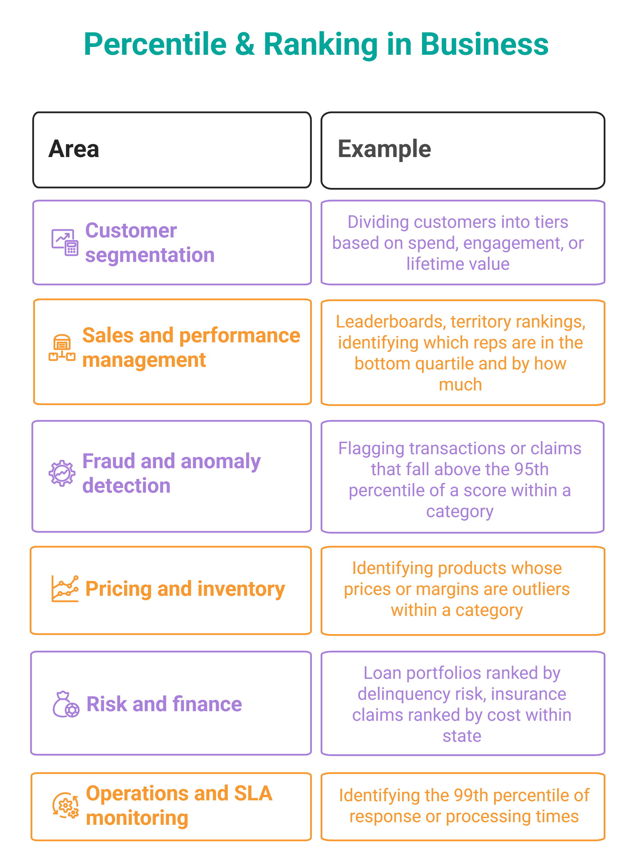
Mixture features let you know the common. Window-based rating features let you know the distribution, and distributions are the place the fascinating enterprise questions dwell. Is your ninetieth percentile order worth unusually excessive, suggesting a couple of giant consumers are skewing income? Are the underside 25% of gross sales reps clustered near the median or far under?
NTILE(n) divides rows into n roughly equal buckets. PERCENT_RANK() expresses every row’s rank as a worth between 0 and 1. CUME_DIST() tells you what fraction of rows have a worth lower than or equal to the present row. And PERCENTILE_CONT() computes the precise worth at a given percentile threshold — helpful if you wish to filter based mostly on a dynamic cutoff slightly than rank inside a end result set.
// Instance: Figuring out Prime Percentile Fraud
Here is one by Google and Netflix. They need you to establish probably the most suspicious claims in every state. The belief is that the highest 5% of claims in every state are doubtlessly fraudulent.
Knowledge: The desk is known as fraud_score.
| policy_num | state | claim_cost | fraud_score |
|---|---|---|---|
| ABCD1001 | CA | 4113 | 0.61 |
| ABCD1002 | CA | 3946 | 0.16 |
| ABCD1003 | CA | 4335 | 0.01 |
| … | … | … | … |
| ABCD1400 | TX | 3922 | 0.59 |
Code: Within the code, PERCENTILE_CONT(0.95) computes the interpolated worth on the ninety fifth percentile of fraud scores inside every state.
Within the following SELECT assertion, the CTE is joined with the unique desk so each declare may be in contrast in opposition to the edge for its personal state. Claims at or above that worth make the lower.
WITH state_percentiles AS (
    SELECT state,
           PERCENTILE_CONT(0.95) WITHIN GROUP (ORDER BY fraud_score) AS p95
    FROM fraud_score
    GROUP BY state)
SELECT f.policy_num,
       f.state,
       f.claim_cost,
       f.fraud_score
FROM fraud_score f
JOIN state_percentiles sp
ON f.state = sp.state
WHERE f.fraud_score >= sp.p95;
Output:
| policy_num | state | claim_cost | fraud_score |
|---|---|---|---|
| ABCD1016 | CA | 1639 | 0.96 |
| ABCD1021 | CA | 4898 | 0.95 |
| ABCD1027 | CA | 2663 | 0.99 |
| … | … | … | … |
| ABCD1398 | TX | 3191 | 0.98 |
# Conclusion
These 4 patterns share a typical philosophy: do the work within the database, in a single go the place doable, utilizing the total expressive energy of the SQL window specification.
What makes window features genuinely highly effective is not any single perform in isolation. It is the composability: you possibly can chain CTEs, apply a number of window features in the identical SELECT, and construct complicated analytical logic that reads practically like an outline of the enterprise downside itself.
Nate Rosidi is an information scientist and in product technique. He is additionally an adjunct professor instructing analytics, and is the founding father of StrataScratch, a platform serving to knowledge scientists put together for his or her interviews with actual interview questions from prime firms. Nate writes on the most recent tendencies within the profession market, offers interview recommendation, shares knowledge science initiatives, and covers all the things SQL.

