
That is an try at reproducing the evaluation of Part 2.7 of Bayesian Knowledge Evaluation, third version (Gelman et al.), on kidney most cancers charges within the USA within the Nineteen Eighties. I’ve achieved my finest to wash the info from the unique. Andrew wrote a weblog put up to “disillusion [us] in regards to the reproducibility of textbook evaluation”, wherein he refers to this instance. This may then be an try at reillusionment…
The cleaner information are on GitHub, as is the RMarkDown of this evaluation.
library(usmap)
library(ggplot2)
d = learn.csv("KidneyCancerClean.csv", skip=4)
Within the information, the columns dc and dc.2 correspond (I believe) to the dying counts attributable to kidney most cancers in every county of the USA, respectively in 1908-84 and 1985-89. The columns pop and pop.2 are some measure of the inhabitants within the counties. It’s not clear to me what the opposite columns characterize.
Easy mannequin
Let be the inhabitants on county 


d$dct = d$dc + d$dc.2
d$popm = (d$pop + d$pop.2) / 2
d$thetahat = d$dct / d$popm
Specifically, the unique query is to grasp these two maps, which present the counties within the first and final decile for kidney most cancers deaths.
q = quantile(d$thetahat, c(.1, .9))
d$cancerlow = d$thetahat <= q[1] d$cancerhigh = d$thetahat >= q[2]
plot_usmap("counties", information=d, values="cancerhigh") +
  scale_fill_discrete(h.begin = 200,
                      identify = "Massive fee of kidney most cancers deaths")

plot_usmap("counties", information=d, values="cancerlow") +
  scale_fill_discrete(h.begin = 200,
                      identify = "Low fee of kidney most cancers deaths")
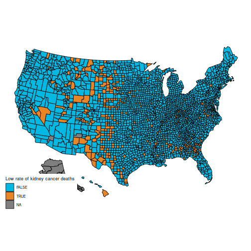
These maps are suprising, as a result of the counties with the best kidney most cancers dying fee, and people with the bottom, are considerably comparable: principally counties in the midst of the map.
(Additionally, be aware that the info for Alaska are lacking. You may conceal Alaska on the maps by including the parameter embrace = statepop$full[-2] to calls to plot_usmap.)
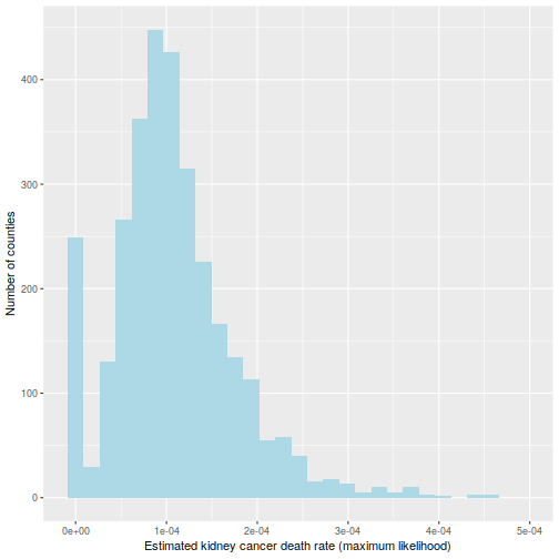
The rationale for this sample (as defined in BDA3) is that these are counties with a low inhabitants. Certainly, a typical worth for 


That is hinted at on this histogram of the 
ggplot(information=d, aes(d$thetahat)) +
  geom_histogram(bins=30, fill="lightblue") +
  labs(x="Estimated kidney most cancers dying fee (most chance)",
       y="Variety of counties") +
  xlim(c(-1e-5, 5e-4))
Bayesian strategy
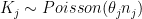
When you have ever adopted a Bayesian modelling course, you might be in all probability screaming that this requires a hierarchical mannequin. I agree (and I’m fairly certain the authors of BDA do as effectively), however here’s a extra primary Bayesian strategy. Take a standard 


The prior is conjugate, so the posterior is 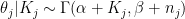
It’s often a disgrace to make use of solely level estimates, however right here it is going to be enough: allow us to compute the posterior imply of
alpha = 15
beta = 2e5
d$thetabayes = (alpha + d$dct) / (beta + d$pop)
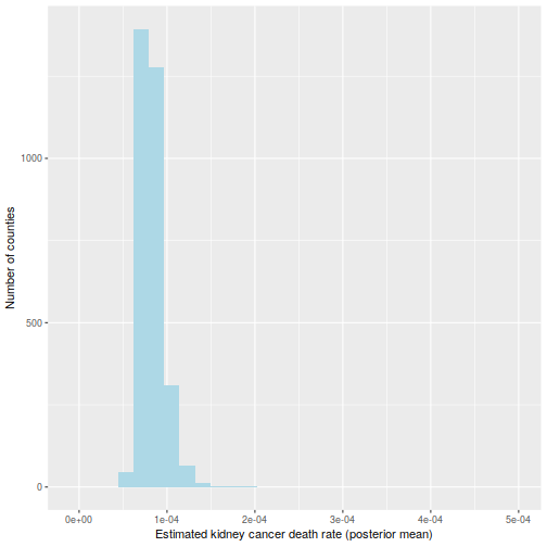
ggplot(information=d, aes(d$thetabayes)) +
geom_histogram(bins=30, fill="lightblue") +
labs(x="Estimated kidney most cancers dying fee (posterior imply)",
y="Variety of counties") +
xlim(c(-1e-5, 5e-4))
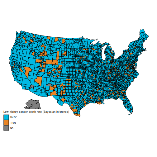
And the maps of counties within the first and final decile are actually a lot simpler to differentiate; as an example, Florida and New England are closely represented within the final decile. The counties represented listed here are principally populated counties: these are counties for which we’ve got cause to imagine that they’re on the decrease or increased finish for kidney most cancers dying charges.
qb = quantile(d$thetabayes, c(.1, .9))
d$bayeslow = d$thetabayes <= qb[1] d$bayeshigh = d$thetabayes >= qb[2]
plot_usmap("counties", information=d, values="bayeslow") +
  scale_fill_discrete(
    h.begin = 200,
    identify = "Low kidney most cancers dying fee (Bayesian inference)")
plot_usmap("counties", information=d, values="bayeshigh") +
  scale_fill_discrete(
    h.begin = 200,
    identify = "Excessive kidney most cancers dying fee (Bayesian inference)")
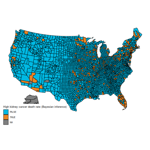
An necessary caveat: I’m not an knowledgeable on most cancers charges (and I count on a few of the vocabulary I used is ill-chosen), nor do I declare that the info listed here are appropriate (from what I perceive, many changes should be made, however they aren’t detailed in BDA, which explains why the maps are barely totally different). I’m merely posting this as a reproducible instance the place the naïve frequentist and Bayesian estimators differ appreciably, as a result of they deal with pattern dimension in numerous methods. I’ve discovered this instance to be helpful in introductory Bayesian programs, because the distinction is straightforward to understand for college kids who’re new to Bayesian inference.