

Technically, at present’s submit has nothing to do with Claude Code. It’s purely algebraic Frisch-Waugh-Lovell, and thus as a result of it’s about steady therapy diff-in-diff, it suits underneath the diff-in-diff banner, and due to this fact is topic to my randomized paywall. So I flipped a coin 3 times, it got here up heads twice, due to this fact it’s paywalled. And so paywalled it shall be. However first, let me inform you what you’re going to be lacking in case you are not a paying subscriber.
I’m going to stroll us by way of the FWL decomposition of a TWFE regression coefficient. The TWFE regression coefficient is a regression of some final result onto unit and time fastened results for 2 durations and a steady dosage variable. Consider the dose because the minimal wage. We aren’t, in different phrases, simply considering of whether or not a municipality raises the minimal wage — which might be a binary therapy. We’re serious about how a lot which is a steady measure of therapy. So after I say “dosage”, I imply “a selected worth of some therapy”. That is the decomposition in Desk 1 of Callaway, Goodman-Bacon and Sant’Anna (CBS).
Thanks once more for all of your assist. Right this moment is the day that you could be need to grow to be a subscriber as a result of at present is the day that we attempt to determine what’s underneath the hood for TWFE with steady dose.
I’m going to be on this part going from a regression components, which you’ll consider because the inhabitants regression from which we are going to get a greatest linear predictor (BLP) inhabitants coefficient estimated with two-way fastened results (TWFE), to one of many 4 decompositions in Desk 1 of CBS. This half is sluggish as a result of I must grasp this for my very own sake, and I would like the steps spelled out for me, and I’m utilizing the substack to mainly go sluggish.
So let’s begin with the regression itself.
(y_{i,t} = α_i + β^{twfe} D_i cdot Post_t + λ_t + ε_{i,t})
the place i indexes models, t indexes pre and submit, D is the continual time-invariant dose, and Publish is a dummy that activates in interval 2. The “time-invariant” is operationalizing a two-period diff-in-diff the place at baseline, Publish=0, it cancels out totally, and it’s canceling out for the comparability unit too, D=0. However for handled models within the submit interval, the dose “activates”. They’ve extra common extensions, however we begin with this dosage group, D, occasions T, as that’s the equal of the 2×2 for individuals who know the fashionable diff-in-diff literature.
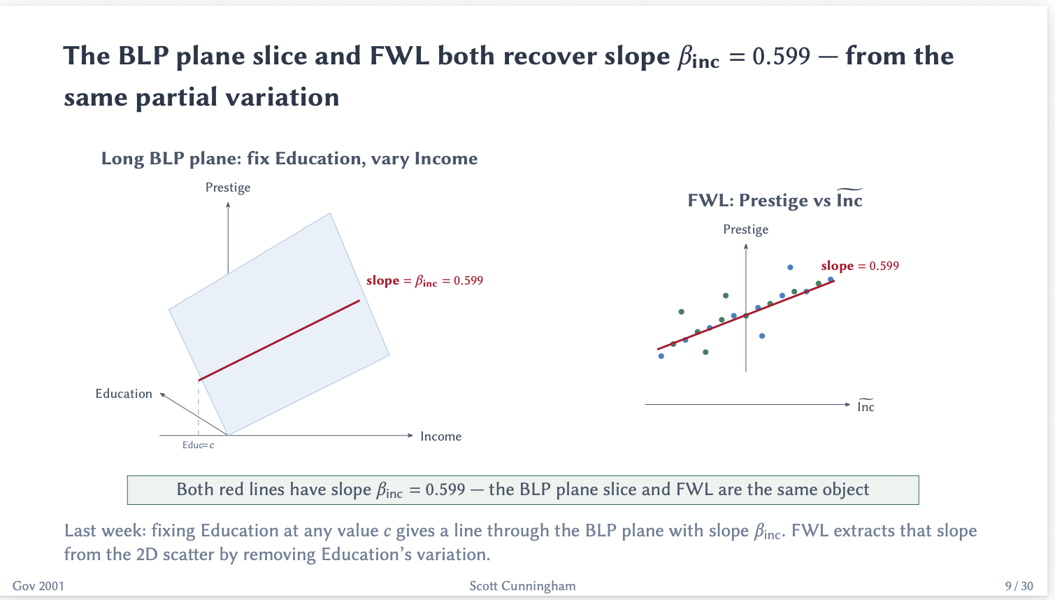
We begin by utilizing Frisch-Waugh-Lovell to residualize the beta coefficient (technically as soon as calculated this turns into the BLP). You possibly can see my lectures on FWL from earlier this week in my Gov 2001 class at Harvard on chance and statistics, additionally, if you wish to see extra about it, however FWL partials out covariates and turns a multi-variate regression slope right into a univariate one. In our case the covariates are the time and unit fastened results. So with some algebra expressing numerous demeaning, that regression coefficient is:
({;beta^{textual content{twfe}} ;=; frac{sum_i (D_i – bar{D})(Delta y_i – overline{Delta y})}{sum_i (D_i – bar{D})^2} ;=; frac{widehat{textual content{Cov}}(D_i,, Delta y_i)}{widehat{textual content{Var}}(D_i)}.;})
That’s the BLP regression coefficient with a steady D x Publish interplay having been residualized by FWL right into a univariate slope, like I mentioned and it’s mechanically nothing greater than the OLS slope of the unit-level first distinction on the dose. I don’t have a visible of this itself, however I do have a visualization of this with two covariates (making a BLP that could be a aircraft) that by way of FWL turns into a univariate slope from my Gov 2001 lecture slides this week, simply so you’ll be able to see. By allegory, the left image right here can be the multivariate regression coefficient from the primary equation (word that the slope of the aircraft is similar for all covariate values, therefore “holding fixed”) and the image on the fitting is the univariate slope itself. All that FWL does is rip out the slope and recast it, however in our case it would additionally lead us to the decompositions we care about.
Right here is the decomposition I’m centered on from Desk 1 of CBS. For at present, I’ll solely be concentrating on the “Ranges” row although. That’s row 2 for the optimistic dose weights (column 1) and the zero dose weights (column 2).
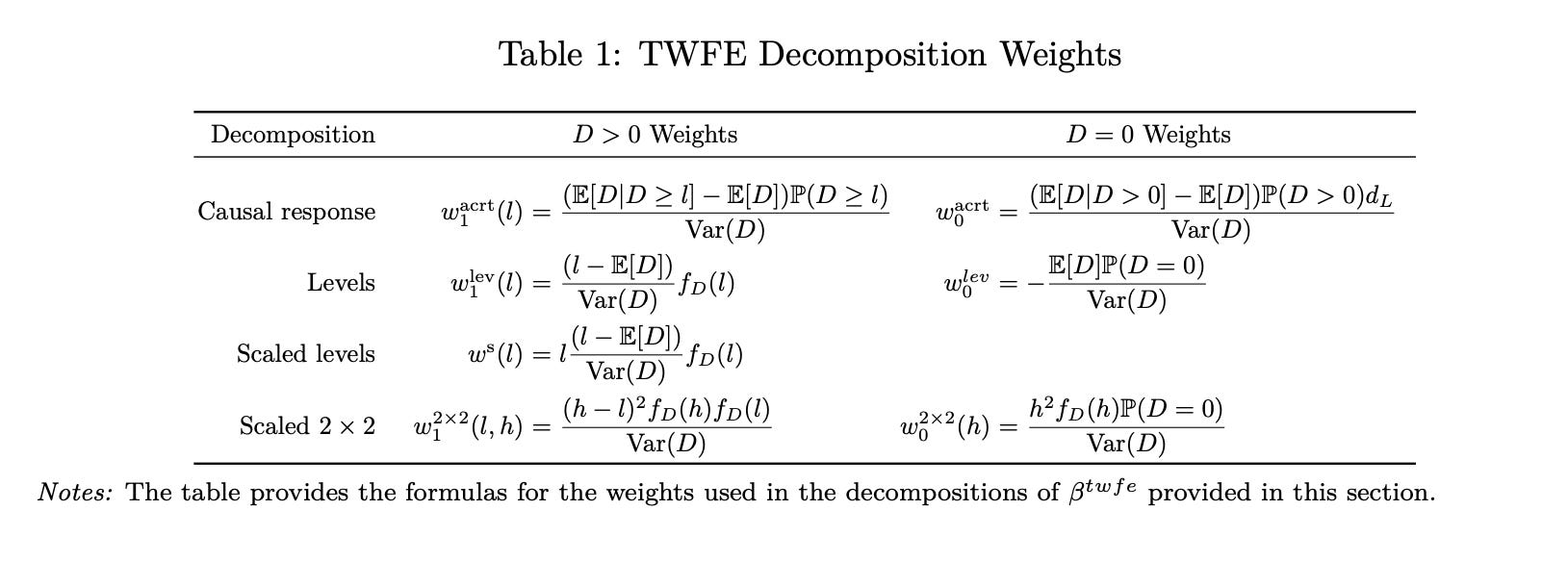
So, choosing again up the place I left off, to get to our ranges decomposition, I begin by conditioning on D by iterated expectations which causes the dose distribution to separate into its level mass at zero, weight P(D=0), and its steady half on the density of D on the optimistic assist vary (word: dose can not grow to be detrimental; simply solely 0 or >0).