

In my final posting, I launched you to the ideas of hierarchical or “multilevel” information. In as we speak’s publish, I’d like to point out you easy methods to use multilevel modeling methods to analyse longitudinal information with Stata’s xtmixed command.
Final time, we seen that our information had two options. First, we seen that the means inside every degree of the hierarchy had been totally different from one another and we included that into our information evaluation by becoming a “variance part” mannequin utilizing Stata’s xtmixed command.
The second function that we seen is that repeated measurement of GSP confirmed an upward development. We’ll decide up the place we left off final time and stick with the ideas once more and you’ll consult with the references on the finish to be taught extra in regards to the particulars.
The movies
Stata has a really pleasant dialog field that may help you in constructing multilevel fashions. If you want a short introduction utilizing the GUI, you may watch an indication on Stata’s YouTube Channel:
Introduction to multilevel linear fashions in Stata, half 2: Longitudinal information
Longitudinal information
I’m typically requested by starting information analysts – “What’s the distinction between longitudinal information and time-series information? Aren’t they the identical factor?”.
The confusion is comprehensible — each sorts of information contain some measurement of time. However the reply isn’t any, they aren’t the identical factor.
Univariate time collection information sometimes come up from the gathering of many information factors over time from a single supply, similar to from an individual, nation, monetary instrument, and so on.
Longitudinal information sometimes come up from accumulating a couple of observations over time from many sources, similar to a couple of blood stress measurements from many individuals.
There are some multivariate time collection that blur this distinction however a rule of thumb for distinguishing between the 2 is that point collection have extra repeated observations than topics whereas longitudinal information have extra topics than repeated observations.
As a result of our GSP information from final time contain 17 measurements from 48 states (extra sources than measurements), we are going to deal with them as longitudinal information.
GSP Information: http://www.stata-press.com/information/r12/productiveness.dta
Random intercept fashions
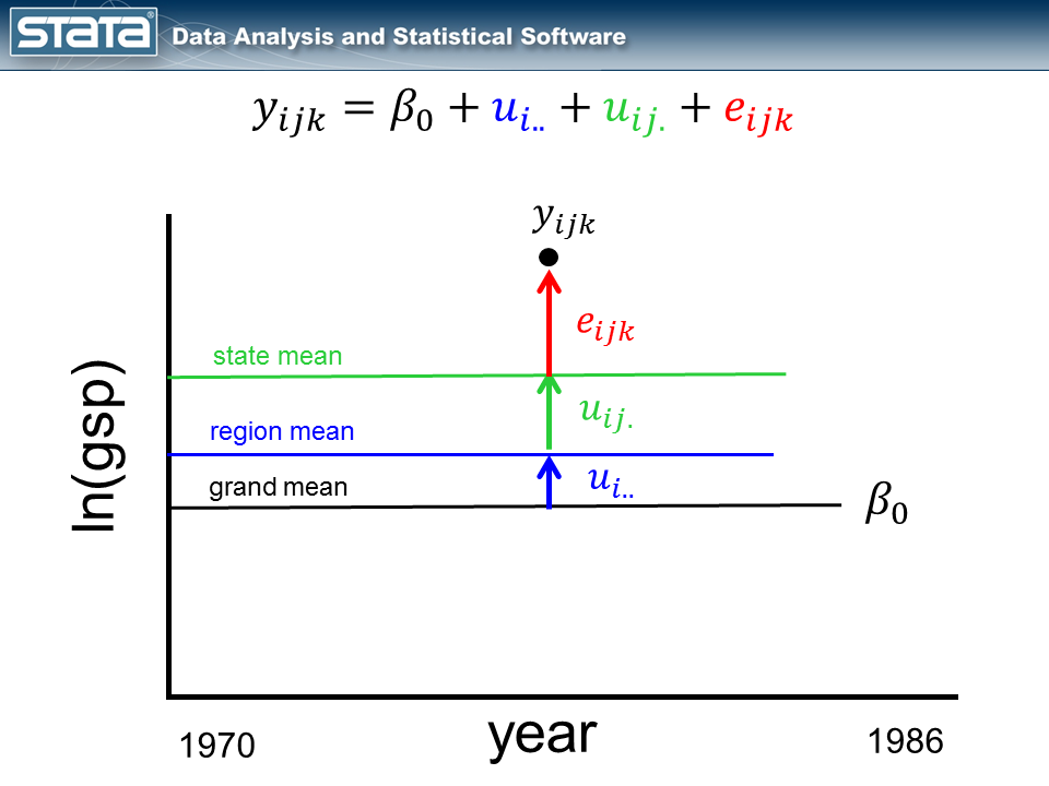
As I discussed final time, repeated observations on a gaggle of people may be conceptualized as multilevel information and modeled simply as every other multilevel information. We left off final time with a variance part mannequin for GSP (Gross State Product, logged) and famous that our mannequin assumed a relentless GSP over time whereas the information confirmed a transparent upward development.
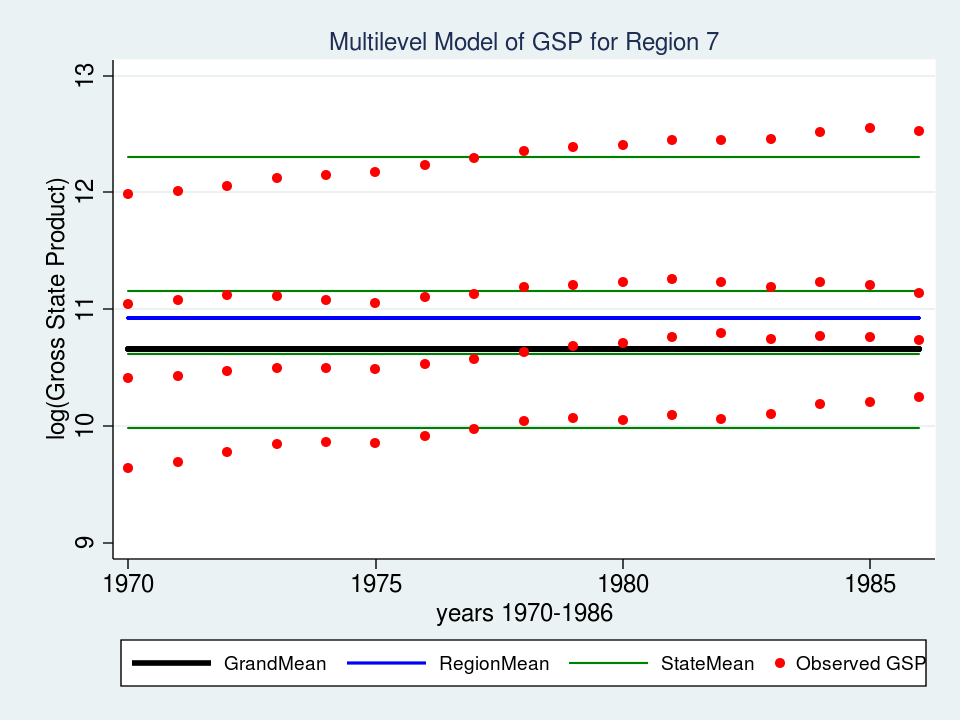
If we think about a single statement and take into consideration our mannequin, nothing within the fastened or random a part of the fashions is a perform of time.
Let’s start by including the variable yr to the fastened a part of our mannequin.
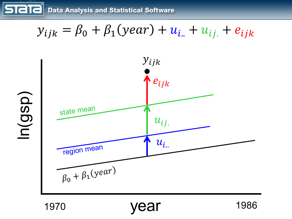
As we anticipated, our grand imply has develop into a linear regression which extra precisely displays the change over time in GSP. What could be surprising is that every state’s and area’s imply has modified as properly and now has the identical slope because the regression line. It’s because not one of the random elements of our mannequin are a perform of time. Let’s match this mannequin with the xtmixed command:
. xtmixed gsp yr, || area: || state:

------------------------------------------------------------------------------
         gsp |      Coef.   Std. Err.      z    P>|z|     [95% Conf. Interval]
-------------+----------------------------------------------------------------
        yr |   .0274903   .0005247    52.39   0.000     .0264618    .0285188
       _cons |  -43.71617   1.067718   -40.94   0.000    -45.80886   -41.62348
------------------------------------------------------------------------------

------------------------------------------------------------------------------
  Random-effects Parameters  |   Estimate   Std. Err.     [95% Conf. Interval]
-----------------------------+------------------------------------------------
area: Identification             |
                   sd(_cons) |   .6615238   .2038949      .3615664    1.210327
-----------------------------+------------------------------------------------
state: Identification              |
                   sd(_cons) |   .7805107   .0885788      .6248525    .9749452
-----------------------------+------------------------------------------------
                sd(Residual) |   .0734343   .0018737      .0698522    .0772001
------------------------------------------------------------------------------
The fastened a part of our mannequin now shows an estimate of the intercept (_cons = -43.7) and the slope (yr = 0.027). Let’s graph the mannequin for Area 7 and see if it suits the information higher than the variance part mannequin.
predict GrandMean, xb
label var GrandMean "GrandMean"
predict RegionEffect, reffects degree(area)
predict StateEffect, reffects degree(state)
gen RegionMean = GrandMean + RegionEffect
gen StateMean = GrandMean + RegionEffect + StateEffect

twoway  (line GrandMean yr, lcolor(black) lwidth(thick))      ///
        (line RegionMean yr, lcolor(blue) lwidth(medthick))   ///
        (line StateMean yr, lcolor(inexperienced) join(ascending)) ///
        (scatter gsp yr, mcolor(crimson) msize(medsmall))         ///
        if area ==7,                                          ///
        ytitle(log(Gross State Product), margin(medsmall))      ///
        legend(cols(4) measurement(small))                             ///
        title("Multilevel Mannequin of GSP for Area 7", measurement(medsmall))
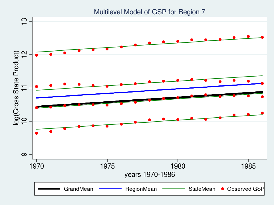
That appears like a a lot better match than our variance-components mannequin from final time. Maybe I ought to depart properly sufficient alone, however I can’t assist noticing that the slopes of the inexperienced traces for every state don’t match in addition to they may. The highest inexperienced line suits properly however the second from the highest appears prefer it slopes upward greater than is critical. That’s the most effective match we will obtain if the regression traces are pressured to be parallel to one another. However what if the traces weren’t pressured to be parallel? What if we may match a “mini-regression mannequin” for every state inside the context of my general multilevel mannequin. Effectively, excellent news — we will!
Random slope fashions
By introducing the variable yr to the fastened a part of the mannequin, we turned our grand imply right into a regression line. Subsequent I’d like to include the variable yr into the random a part of the mannequin. By introducing a fourth random part that could be a perform of time, I’m successfully estimating a separate regression line inside every state.
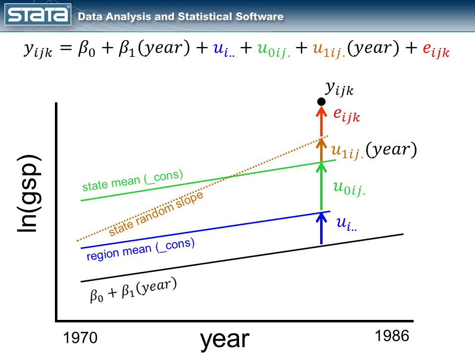
Discover that the scale of the brand new, brown deviation u1ij. is a perform of time. If the statement had been one yr to the left, u1ij. could be smaller and if the statement had been one yr to the appropriate, u1ij.could be bigger.
It is not uncommon to “heart” the time variable earlier than becoming these sorts of fashions. Explaining why is for one more day. The short reply is that, sooner or later through the becoming of the mannequin, Stata should compute the equal of the inverse of the sq. of yr. For the yr 1986 this seems to be 2.535e-07. That’s a reasonably small quantity and if we multiply it by one other small quantity…properly, you get the thought. By centering age (e.g. cyear = yr – 1978), we get a extra affordable quantity for 1986 (0.01). (Trace: You probably have issues along with your mannequin converging and you’ve got massive values for time, strive centering them. It gained’t all the time assist, however it may).
So let’s heart our yr variable by subtracting 1978 and match a mannequin that features a random slope.
gen cyear = yr - 1978
xtmixed gsp cyear, || area: || state: cyear, cov(indep)
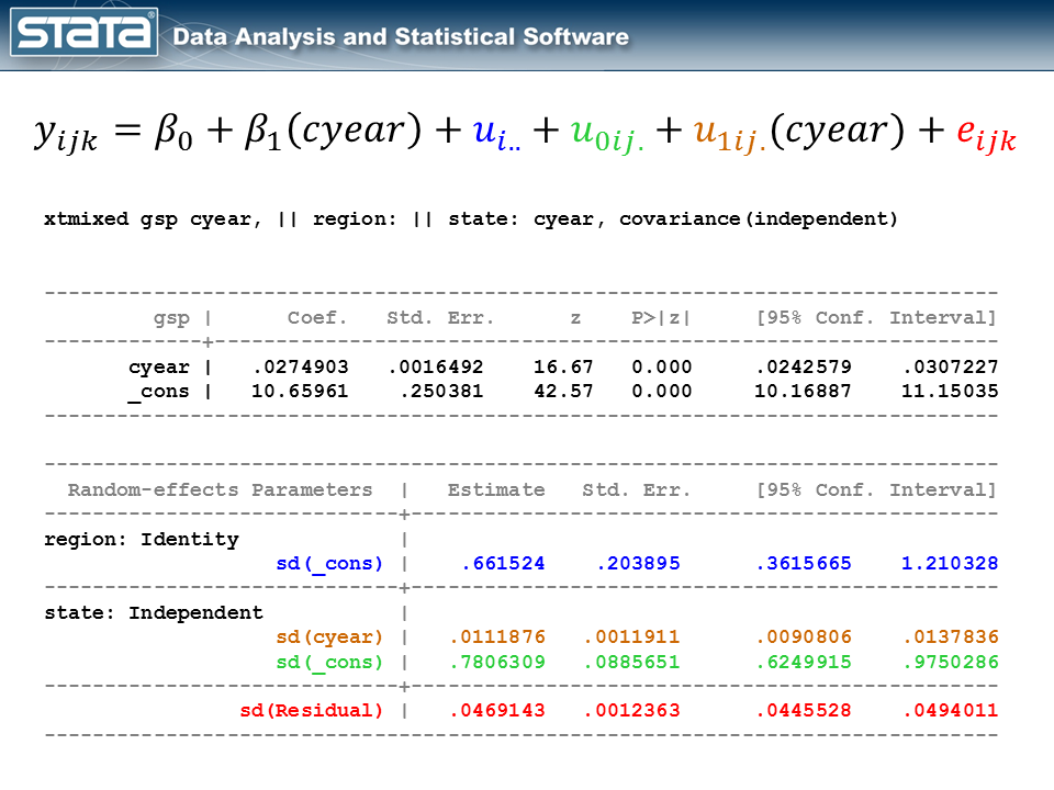
I’ve color-coded the output in order that we will match every a part of the output again to the mannequin and the graph. The fastened a part of the mannequin seems within the prime desk and it appears like every other easy linear regression mannequin. The random a part of the mannequin is unquestionably extra sophisticated. Should you get misplaced, look again on the graphic of the deviations and remind your self that we have now merely partitioned the deviation of every statement into 4 elements. If we did this for each statement, the usual deviations in our output are merely the common of these deviations.
Let’s take a look at a graph of our new “random slope” mannequin for Area 7 and see how properly it suits our information.
predict GrandMean, xb
label var GrandMean "GrandMean"
predict RegionEffect, reffects degree(area)
predict StateEffect_year StateEffect_cons, reffects degree(state)

gen RegionMean = GrandMean + RegionEffect
gen StateMean_cons = GrandMean + RegionEffect + StateEffect_cons
gen StateMean_year = GrandMean + RegionEffect + StateEffect_cons + ///
                     (cyear*StateEffect_year)

twoway  (line GrandMean cyear, lcolor(black) lwidth(thick))             ///
        (line RegionMean cyear, lcolor(blue) lwidth(medthick))          ///
        (line StateMean_cons cyear, lcolor(inexperienced) join(ascending))   ///
        (line StateMean_year cyear, lcolor(brown) join(ascending))   ///
        (scatter gsp cyear, mcolor(crimson) msize(medsmall))                ///
        if area ==7,                                                  ///
        ytitle(log(Gross State Product), margin(medsmall))              ///
        legend(cols(3) measurement(small))                                     ///
        title("Multilevel Mannequin of GSP for Area 7", measurement(medsmall))
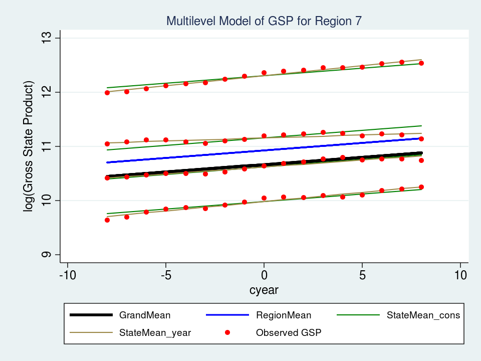
The highest brown line suits the information barely higher, however the brown line under it (second from the highest) is a a lot better match. Mission completed!
The place can we go from right here?
I hope I’ve been capable of persuade you that multilevel modeling is straightforward utilizing Stata’s xtmixed command and that this can be a software that it would be best to add to your equipment. I might like to say one thing like “And that’s all there may be to it. Go forth and construct fashions!”, however I might be remiss if I didn’t level out that I’ve glossed over many essential matters.
In our GSP instance, we might nonetheless like to think about the impression of different unbiased variables. I haven’t talked about alternative of estimation strategies (ML or REML within the case of xtmixed). I’ve assessed the match of our fashions by graphs, an strategy essential however incomplete. We haven’t thought of speculation testing. Oh — and, all the standard residual diagnostics for linear regression similar to checking for outliers, influential observations, heteroskedasticity and normality nonetheless apply….occasions 4! However now that you just perceive the ideas and a few of the mechanics, it shouldn’t be troublesome to fill within the particulars. Should you’d prefer to be taught extra, try the hyperlinks under.
I hope this was useful…thanks for stopping by.
For extra data
Should you’d prefer to be taught extra about modeling multilevel and longitudinal information, try
Multilevel and Longitudinal Modeling Utilizing Stata, Third Version
Quantity I: Steady Responses
Quantity II: Categorical Responses, Counts, and Survival
by Sophia Rabe-Hesketh and Anders Skrondal
or join our widespread public coaching course Multilevel/Blended Fashions Utilizing Stata.