

Introduction
Right this moment I wish to present you how you can create animated graphics utilizing Stata. It’s simpler than you may count on and you should use animated graphics as an example ideas that may be difficult as an example with static graphs. Along with Stata, you will have a video modifying program however don’t be involved in case you don’t have one. On the 2012 UK Stata Person Group Assembly Robert Grant demonstrated how you can create animated graphics from inside Stata utilizing a free software program program known as FFmpeg. I’ll present you the way I create my animated graphs utilizing Camtasia and the way Robert creates his utilizing FFmpeg.
I lately recorded a video for the Stata Youtube channel known as “Energy and pattern measurement calculations in Stata: A conceptual introduction“. I needed as an example two ideas: (1) that statistcal energy will increase as pattern measurement will increase, and (2) as impact measurement will increase. Each of those ideas could be illustrated with a static graph together with the reason “think about that …”. Creating animated graphs allowed me to skip the reason and simply present what I meant.
Creating the graphs
Movies are illusions. All movies — from Charles-Émile Reynaud’s 1877 praxinoscope to trendy blu-ray films — are created by displaying a collection of ordered nonetheless pictures for a fraction of a second every. Our brains understand this collection of nonetheless pictures as movement.
To create the phantasm of movement with graphs, we make an ordered collection of barely differing graphs. We will use loops to do that. If you’re not conversant in loops in Stata, right here’s one to rely to 5:
forvalues i = 1(1)5 {
    disp "i = `i'"
}

i = 1
i = 2
i = 3
i = 4
i = 5
We may place a graph command contained in the loop. If, for every interation, the graph command created a barely completely different graph, we might be on our method to creating our first video. The loop under creates a collection of graphs of regular densities with means 0 by 1 in increments of 0.1.
forvalues mu = 0(0.1)1 {
    twoway  perform y=normalden(x,`mu',1), vary(-3 6) title("N(`mu',1)")
}
You could have seen the phantasm of movement as Stata created every graph; the conventional densities seemed to be shifting to the correct as every new graph appeared on the display.
You could have additionally seen that a number of the values of the imply didn’t look as you’ll have needed. For instance, 1.0 was displayed as 0.999999999. That’s not a mistake, it’s as a result of Stata shops numbers and performs calculations in base two and shows them in base ten; for an in depth clarification, see Precision (but once more), Half I.
We will repair that by reformating the means utilizing the string() perform.
forvalues mu = 0(0.1)1 {
    native mu = string(`mu', "%3.1f")
    twoway  perform y=normalden(x,`mu',1), vary(-3 6) title("N(`mu',1)")
}
Subsequent, we have to save our graphs. We will do that by including graph export contained in the loop.
forvalues mu = 0(0.1)1 {
    native mu = string(`mu', "%3.1f")
    twoway  perform y=normalden(x,`mu',1), vary(-3 6) title("N(`mu',1)")
    graph export graph_`mu'.png, as(png) width(1280) peak(720) substitute
}
Notice that the title of every graph file contains the worth of mu in order that we all know the order of our information. We will view the contents of the listing to confirm that Stata has created a file for every of our graphs.
. ls2/11/14 12:12 . 2/11/14 12:12 .. 35.6k 2/11/14 12:11 graph_0.0.png 35.6k 2/11/14 12:11 graph_0.1.png 35.7k 2/11/14 12:11 graph_0.2.png 35.7k 2/11/14 12:11 graph_0.3.png 35.7k 2/11/14 12:11 graph_0.4.png 35.8k 2/11/14 12:11 graph_0.5.png 35.9k 2/11/14 12:12 graph_0.6.png 35.7k 2/11/14 12:12 graph_0.7.png 35.8k 2/11/14 12:12 graph_0.8.png 35.9k 2/11/14 12:12 graph_0.9.png 35.6k 2/11/14 12:12 graph_1.0.png
Now that we’ve got created our graphs, we have to mix them right into a video.
There are a lot of industrial, freeware, and free software program applications out there that we may use. I’ll define the essential steps utilizing two of them, one a commerical GUI primarily based product (not free) known as Camtasia, and the opposite a free command-based program known as FFmpeg.
Creating movies with Camtasia
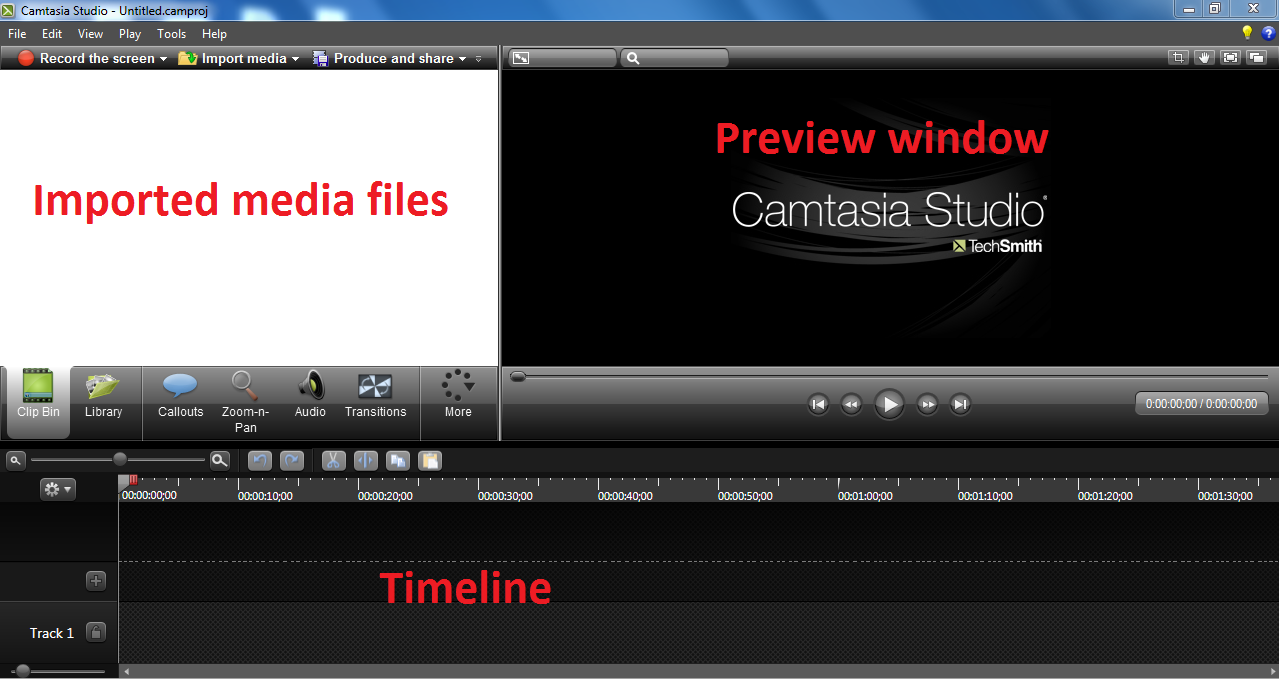
Most industrial video modifying applications have related interfaces. The person imports picture, sound and video information, organizes them in tracks on a timeline after which previews the ensuing video. Camtasia is a industrial video program that I exploit to file movies for the Stata Youtube channel and its interface seems to be like this.
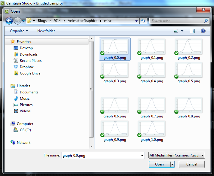
We start by importing the graph information into Camtasia:
Subsequent we drag the pictures onto the timeline:
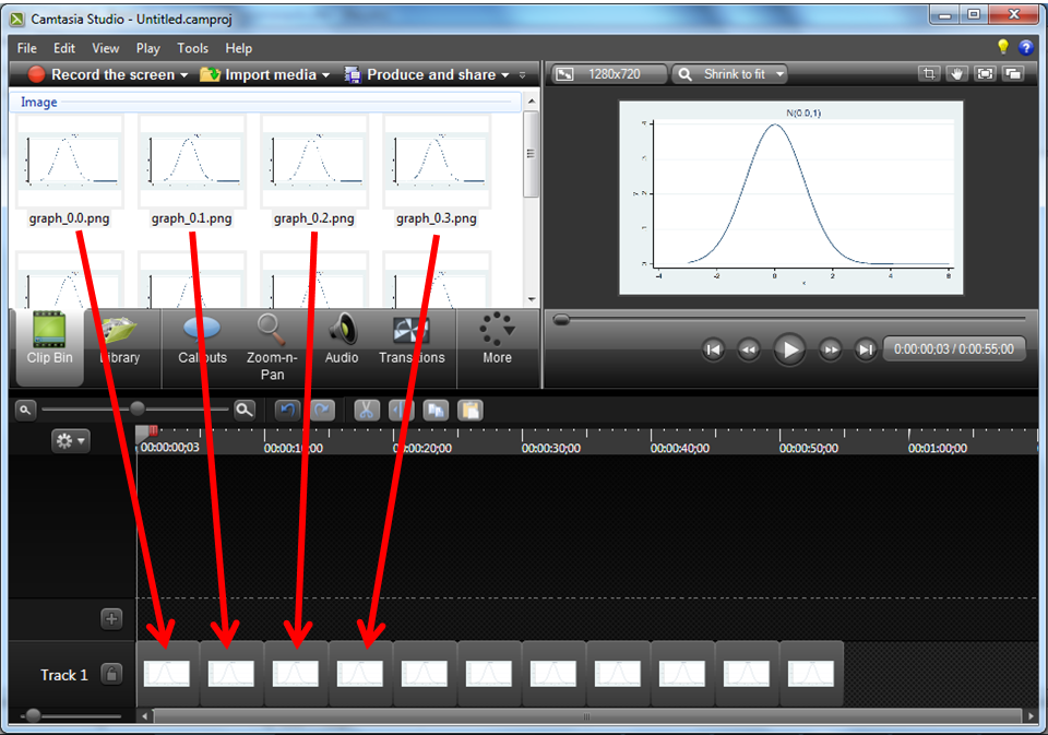
After which we make the show time for every picture very quick…on this case 0.1 seconds or 10 frames per second.
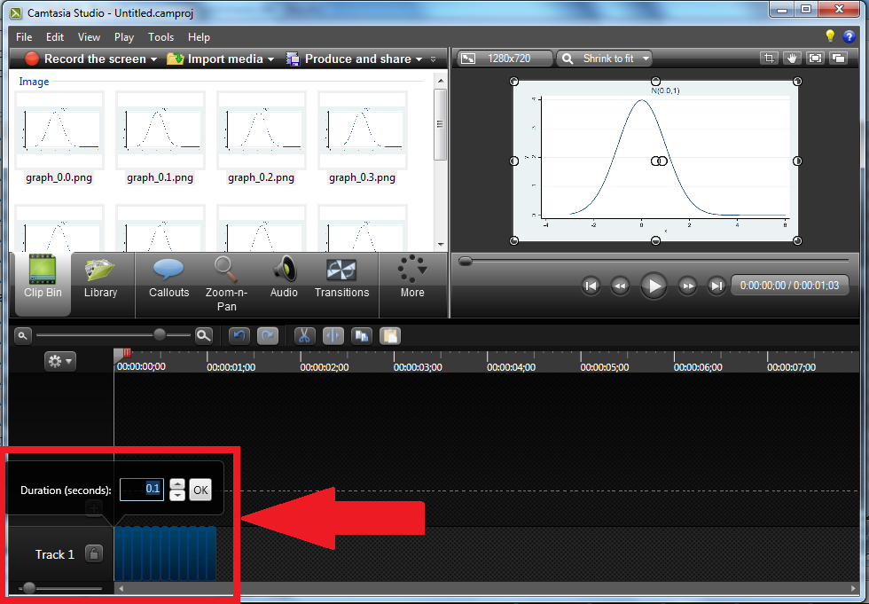
After previewing the video, we are able to export it to any of Camtasia’s supported codecs. I’ve exported to a “.gif” file as a result of it’s straightforward to view in an online browser.
We simply created our first animated graph! All we’ve got to do to make it look as skilled because the power-and-sample measurement examples I confirmed you earlier is return into our Stata program and modify the graph command so as to add the extra parts we wish to show!
Creating movies with FFmpeg
Stata person and medical statistician Robert Grant gave a presentation on the 2012 UK Stata Person Group Assembly in London entitled “Producing animated graphs from Stata with out having to be taught any specialised software program“. You’ll be able to learn extra about Robert by visiting his weblog and clicking on About.
In his presentation, Robert demonstrated how you can mix graph pictures right into a video utilizing a free software program program known as FFmpeg. Robert adopted the identical fundamental technique I demonstrated above, however Robert’s alternative of software program has two interesting options. First, the software program is available and free. Second, FFmpeg could be known as from throughout the Stata surroundings utilizing the winexec command. Which means that we are able to create our graphs and mix them right into a video utilizing Stata do information. Combining dozens or a whole lot of graphs right into a single video with a program is quicker and simpler than utilizing a drag-and-drop interface.
Let’s return to our earlier instance and mix the information utilizing FFmpeg. Recall that we inserted the imply into the title of every file (e.g. “graph_0.4.png”) in order that we may preserve observe of the order of the information. In my expertise, it may be troublesome to mix information with decimals of their names utilizing FFmpeg. To keep away from the issue, I’ve added a line of code between the twoway command and the graph export command that names the information with sequential integers that are padded with zeros.
forvalues mu = 0(0.1)1 {
    native mu = string(`mu', "%3.1f")
    twoway perform y=normalden(x,`mu',1), vary(-3 6) title("N(`mu',1)")
    native mu = string(`mu'*10+1, "%03.0f")
    graph export graph_`mu'.png, as(png) width(1280) peak(720) substitute
}

. ls
     2/12/14 12:21  .
     2/12/14 12:21  ..
  35.6k   2/12/14 12:21  graph_001.png
  35.6k   2/12/14 12:21  graph_002.png
  35.7k   2/12/14 12:21  graph_003.png
  35.7k   2/12/14 12:21  graph_004.png
  35.7k   2/12/14 12:21  graph_005.png
  35.8k   2/12/14 12:21  graph_006.png
  35.9k   2/12/14 12:21  graph_007.png
  35.7k   2/12/14 12:21  graph_008.png
  35.8k   2/12/14 12:21  graph_009.png
  35.9k   2/12/14 12:21  graph_010.png
  35.6k   2/12/14 12:21  graph_011.png
We will then mix these information right into a video with FFmpeg utilizing the next instructions
native GraphPath "C:UsersjchAnimatedGraphicsexample"
winexec "C:Program FilesFFmpegbinffmpeg.exe" -i `GraphPath'graph_percent03d.png
    -b:v 512k `GraphPath'graph.mpg
The native macro GraphPath incorporates the trail for the listing the place my graphics information are saved.
The Stata command winexec “no matter“ executes no matter. In our case, no matter is ffmpeg.exe, preceeded by ffmpeg.exe‘s path, and adopted by the arguments FFmpeg wants. We specify two choices, -i and -b.
The -i choice is adopted by a path and filename template. In our case, the trail is obtained from the Stata native macro GraphPath and the filename template is “graph_percent03d.png”. This template tells FFmpeg to search for a 3 digit sequence of numbers between “graph_” and “.png” within the filenames. The zero that precedes the three within the template tells FFmpeg that the three digit sequence of numbers is padded with zeros.
The -b choice specifies the trail and filename of the video to be created together with some attributes of the video.
As soon as we’ve got created our video, we are able to use FFmpeg to transform our video to different video codecs. For instance, we may convert “graph.mpg” to “graph.gif” utilizing the next command:
winexec "C:Program FilesFFmpegbinffmpeg.exe" -r 10 -i `GraphPath'graph.mpg
    -t 10 -r 10 `GraphPath'graph.gif
which creates this graph:
FFmpeg is a really versatile program and there are far too many choices to debate on this weblog entry. If you need to be taught extra about FFmpeg you may go to their web site at www.ffmpeg.org.
Extra Examples
I made the previous examples so simple as potential in order that we may give attention to the mechanics of making movies. We now know that, if we wish to make skilled trying movies, all of the complication comes on the Stata facet. We go away our loop alone however change the graph command inside it to be extra sophisticated.
So right here’s how I created the 2 animated-graphics movies that I used to create the general video “Energy and pattern measurement calculations in Stata: A conceptual introduction” on our YouTube channel.
The primary demonstrated that rising the impact measurement (the distinction between the means) ends in elevated statistical energy.
native GraphCounter = 100
native mu_null = 0
native sd = 1
native z_crit = spherical(-1*invnormal(0.05), 0.01)
native z_crit_label = `z_crit' + 0.75

forvalues mu_alt = 1(0.01)3 {
  twoway  ///
    perform y=normalden(x,`mu_null',`sd'),                    ///
             vary(-3 `z_crit') shade(pink) dropline(0)   ||    ///
    perform y=normalden(x,`mu_alt',`sd'),                     ///
             vary(-3 5) shade(inexperienced) dropline(`mu_alt') ||    ///
    perform y=normalden(x,`mu_alt',`sd'),                     ///
             vary(`z_crit' 6) recast(space) shade(inexperienced) ||    ///
    perform y=normalden(x,`mu_null',`sd'),                    ///
             vary(`z_crit' 6) recast(space) shade(pink)         ///
    title("Energy for {&mu}={&mu}{subscript:0} versus {&mu}={&mu}{subscript:A}") ///
    xtitle("{it: z}") xlabel(-3 -2 -1 0 1 2 3 4 5 6)           ///
    legend(off)                                                ///
    ytitle("Density") yscale(vary(0 0.6))                     ///
    ylabel(0(0.1)0.6, angle(horizontal) nogrid)                ///
    textual content(0.45 0 "{&mu}{subscript:0}", shade(pink))              ///
    textual content(0.45 `mu_alt' "{&mu}{subscript:A}", shade(inexperienced))

  graph export mu_alt_`GraphCounter'.png, as(png) width(1280) peak(720) substitute

  native ++GraphCounter
}
The above Stata code created the *.png information that I then mixed utilizing Camtasia to provide this gif:
The second video demonstrated that energy will increase because the pattern measurement will increase.
native GraphCounter = 301
native mu_label = 0.45
native power_label = 2.10
native mu_null = 0
native mu_alt = 2

forvalues sd = 1(-0.01)0.5 {
  native z_crit = spherical(-1*invnormal(0.05)*`sd', 0.01)
  native z_crit_label = `z_crit' + 0.75

  twoway                                                                        ///
    perform y=normalden(x,`mu_null',`sd'),                                     ///
             vary(-3 `z_crit') shade(pink) dropline(0)  ||                      ///
    perform y=normalden(x,`mu_alt',`sd'),                                      ///
             vary(-3 5) shade(inexperienced)  dropline(`mu_alt')      ||               ///
    perform y=normalden(x,`mu_alt',`sd'),                                      ///
             vary(`z_crit' 6) recast(space) shade(inexperienced)       ||               ///
    perform y=normalden(x,`mu_null',`sd'),                                     ///
             vary(`z_crit' 6) recast(space) shade(pink)                          ///
    title("Energy for {&mu}={&mu}{subscript:0} versus {&mu}={&mu}{subscript:A}") ///
    xtitle("{it: z}") xlabel(-3 -2 -1 0 1 2 3 4 5 6)                            ///
    legend(off)                                                                 ///
    ytitle("Density") yscale(vary(0 0.6))                                      ///
    ylabel(0(0.1)0.6, angle(horizontal) nogrid)                                 ///
    textual content(`mu_label' 0 "{&mu}{subscript:0}", shade(pink))                         ///
    textual content(`mu_label' `mu_alt' "{&mu}{subscript:A}", shade(inexperienced))
  graph export mu_alt_`GraphCounter'.png, as(png) width(1280) peak(720) substitute

  native ++GraphCounter
  native mu_label = `mu_label' + 0.005
  native power_label = `power_label' + 0.03
}
Simply as beforehand, the above Stata code creates the *.png information that I then mix utilizing Camtasia to provide a gif:
Let me present you some extra examples.
The following instance demonstrates the essential thought of lowess smoothing.
sysuse auto
native WindowWidth = 500
forvalues WindowUpper = 2200(25)5000 {
  native WindowLower = `WindowUpper' - `WindowWidth'
  twoway (scatter mpg weight)                                             ///
    (lowess mpg weight if weight < (`WindowUpper'-250), lcolor(inexperienced))    ///
    (lfit mpg weight if weight>`WindowLower' & weight<`WindowUpper',      ///
         lwidth(medium) lcolor(pink))                                      ///
    , xline(`WindowLower' `WindowUpper', lwidth(medium) lcolor(black))    ///
    legend(on order(1 2 3) cols(3))
  graph export lowess_`WindowUpper'.png, as(png) width(1280) peak(720) substitute
}
The result’s,
The animated graph I created just isn’t but an ideal analogy to what lowess truly does, however it comes shut. It has two issues. The lowess curve modifications exterior of the sliding window, which it shouldn’t and the animation doesn’t illustrate the weighting of the factors throughout the window, say through the use of in a different way sized markers for the factors within the sliding window. Even so, the graph does a much better job than the standard explanaton that one ought to think about sliding a window throughout the scatterplot.
As one more instance, we are able to use animated graphs to exhibit the idea of convergence. There’s a FAQ on the Stata web site written by Invoice Gould that explains the relationship between the chi-squared and F distributions. The animated graph under exhibits that F(d1, d2) converges to d1*χ^2 as d2 goes to infinity:
forvalues df = 1(1)100 {
  twoway perform  y=chi2(2,2*x), vary(0 6) shade(pink) ||                                       ///
    perform y=F(2,`df',x), vary(0 6) shade(inexperienced)                                              ///
    title("Cumulative distributions for {&chi}{sup:2}{sub:df} and {it:F}{subscript:df,df2}")     ///
    xtitle("{it: denominator df}") xlabel(0 1 2 3 4 5 6) legend(off)                             ///
    textual content(0.45 4 "df2 = `df'",  measurement(enormous) shade(black))                                          ///
    legend(on order(1 "{&chi}{sup:2}{sub:df}" 2 "{it:F}{subscript:df,df2}") cols(2) place(5) ring(0))

  native df = string(`df', "%03.0f")
  graph export converge2_`df'.png, as(png) width(1280) peak(720) substitute
}
The t distribution has an analogous relationship with the conventional distribution.
forvalues df = 1(1)100 {
  twoway  perform y=regular(x), vary(-3 3) shade(pink)   ||                     ///
    perform y=t(`df',x), vary(-3 3) shade(inexperienced)                              ///
    title("Cumulative distributions for Regular(0,1) and {it:t}{subscript:df}")  ///
    xtitle("{it: t/z}") xlabel(-3 -2 -1 0 1 2 3) legend(off)                    ///
    textual content(0.45 -2 "df = `df'",  measurement(enormous) shade(black))                         ///
    legend(on order(1 "N(0,1)" 2 "{it:t}{subscript:df}") cols(2) place(5) ring(0))

  native df = string(`df', "%03.0f")
  graph export converge_`df'.png, as(png) width(1280) peak(720) substitute
}
The result’s
Remaining ideas
I’ve realized by trial and error two issues that enhance the standard of my animated graphs. First, observe that the axes of the graphs in a lot of the examples above are explicitly outlined within the graph instructions. That is typically essential to preserve the axes steady from graph to graph. Second, movies have a smoother, larger high quality look when there are various graphs with very small modifications from graph to graph.
I hope I’ve satisfied you that creating animated graphics with Stata is less complicated than you imagined. If the outdated saying that “an image is value a thousand phrases” is true, think about what number of phrases it can save you utilizing animated graphs.
Different assets
Relationship between chi-squared and F distributions
Robert Grant’s weblog and examples
Hans Rosling’s 200 International locations recreated utilizing solely Stata