Construct DeepSeek-V3: Multi-Head Latent Consideration (MLA) Structure

Within the first a part of this collection, we laid the muse by exploring the theoretical underpinnings of DeepSeek-V3 and implementing key configuration parts similar to Rotary Placeal Embeddings (RoPE). That tutorial established how DeepSeek-V3 manages long-range dependencies and units up its structure for environment friendly scaling. By grounding idea in working code, we ensured that readers not solely understood the ideas but additionally noticed how they translate into sensible implementation.

With that groundwork in place, we now flip to certainly one of DeepSeek-V3’s most distinctive improvements: Multi-Head Latent Consideration (MLA). Whereas conventional consideration mechanisms have confirmed remarkably efficient, they usually include steep computational and reminiscence prices. MLA reimagines this core operation by introducing a latent illustration area that dramatically reduces overhead whereas preserving the mannequin’s capacity to seize wealthy contextual relationships.

On this lesson, we’ll break down the speculation behind MLA, discover why it issues, after which implement it step-by-step. This installment continues our hands-on strategy — shifting past summary ideas to sensible code — whereas advancing the broader purpose of the collection: to reconstruct DeepSeek-V3 from scratch, piece by piece, till we assemble and prepare the complete structure.

This lesson is the 2nd of the 6-part collection on Constructing DeepSeek-V3 from Scratch:

DeepSeek-V3 Mannequin: Principle, Config, and Rotary Positional Embeddings
Construct DeepSeek-V3: Multi-Head Latent Consideration (MLA) Structure (this tutorial)
Lesson 3
Lesson 4
Lesson 5
Lesson 6

To find out about DeepSeek-V3 and construct it from scratch, simply maintain studying.

Searching for the supply code to this publish?

Leap Proper To The Downloads Part

The KV Cache Reminiscence Downside in DeepSeek-V3

To know why MLA is revolutionary, we should first perceive the reminiscence bottleneck in Transformer inference. Commonplace multi-head consideration computes:

$text{Attention}(Q, K, V) = text{softmax}left(dfrac{QK^T}{sqrt{d_k}}right)V$ ,

the place $Q, K, V in mathbb{R}^{T times d_text{model}}$ are question, key, and worth matrices for sequence size $T$ . In autoregressive technology (producing one token at a time), we can’t recompute consideration over all earlier tokens from scratch at every step — that will be $O(T^2)$ computation per token generated.

As an alternative, we cache the important thing and worth matrices. When producing token $t$ , we solely compute $Q_t$ (the question for the brand new token), then compute consideration utilizing $Q_t$ and the cached $K_{1:t-1}, V_{1:t-1}$ . This reduces computation from $O(T^2)$ to $O(T)$ per generated token — a dramatic speedup.

Nevertheless, this cache comes at a steep reminiscence value. For a mannequin with $L$ layers, $H$ consideration heads, and head dimension $d_text{head} = d_text{model}/H$ , the KV cache requires:

$text{Memory}_text{KV} = 2 times L times H times d_text{head} times T times text{sizeof}(text{float})$ .

For a mannequin like GPT-3 with 96 layers, 96 heads, 128-head dimensions, and 2048 sequence size, that is:

$2 times 96 times 96 times 128 times 2048 times 2 text{ bytes} = 9.6 text{ GB per sequence}$ .

This implies you possibly can solely serve a handful of customers concurrently on even high-end GPUs. The reminiscence bottleneck is commonly the limiting think about deployment, not computation.

Multi-Head Latent Consideration (MLA): KV Cache Compression with Low-Rank Projections

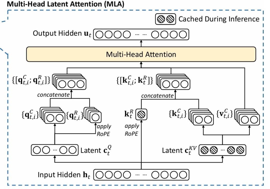
MLA (Determine 1) solves this by means of a compress-decompress technique impressed by Low-Rank Adaptation (LoRA). The important thing perception: we don’t have to retailer full $d_text{model}$ -dimensional representations. We will compress them right into a lower-dimensional latent area for storage, then decompress when wanted for computation.

**Determine 1:** Multi-Head Latent Consideration structure (supply: DeepSeek-AI, 2025).

Step 1. Key-Worth Compression: As an alternative of storing $K, V in mathbb{R}^{T times d_text{model}}$ instantly, we undertaking them by means of a low-rank bottleneck:

$C_{kv} = text{RMSNorm}(X W_text{down}) in mathbb{R}^{T times r_{kv}}$ ,

the place $X in mathbb{R}^{T times d_text{model}}$ is the enter, $W_text{down} in mathbb{R}^{d_text{model} times r_{kv}}$ is the down-projection, and $r_{kv} le d_text{model}$ is the low-rank dimension. We solely cache $C_{kv}$ relatively than the complete $K$ and $V$ .

Step 2. Key-Worth Decompression: Once we want the precise key and worth matrices for consideration computation, we decompress:

$K_text{content} = C_{kv} W_K in mathbb{R}^{T times d_text{model}}$

$V = C_{kv} W_V in mathbb{R}^{T times d_text{model}}$ ,

the place $W_K, W_V in mathbb{R}^{r_{kv} times d_text{model}}$ are up-projection matrices. This decomposition approximates the complete key and worth matrices by means of a low-rank factorization: $K approx X W_text{down} W_K$ and $V approx X W_text{down} W_V$ .

Reminiscence Financial savings: As an alternative of caching $2 times T times d_text{model}$ , we cache $T times r_{kv}$ . The discount issue is $frac{2 times d_text{model}}{r_{kv}}$ . For our configuration with $d_text{model} = 256$ and $r_{kv} = 128$ , it is a 4× discount. For bigger fashions with $d_text{model} = 4096$ and $r_{kv} = 512$ , it’s a 16× discount — transformative for deployment.

Question Compression and Rotary Positional Embeddings (RoPE) Integration

MLA extends compression to queries, although much less aggressively since queries aren’t cached:

$C_q = X W_q in mathbb{R}^{T times r_q}$

$Q_text{content} = C_q W_{Q} in mathbb{R}^{T times d_text{model}}$ ,

the place $r_q$ may be totally different from $r_{kv}$ . In our configuration, $r_q = 192$ versus $r_{kv} = 128$ — we give queries barely extra capability.

Now comes the intelligent half: integrating RoPE. We cut up each queries and keys into content material and positional parts:

$Q = [Q_text{content} parallel Q_text{rope}]$

$K = [K_text{content} parallel K_text{rope}]$ ,

the place $parallel$ denotes concatenation. The content material parts come from the compression-decompression course of described above. The positional parts are separate projections that we apply RoPE to:

$Q_text{rope} = text{RoPE}_m(C_q W{Q_text{rope}})$

$K_text{rope} = text{RoPE}_n(X W{K_text{rope}})$ ,

the place $text{RoPE}_m$ denotes making use of rotary embedding at place $m$ . This separation is essential: content material and place are independently represented and mixed solely within the consideration scores.

Consideration Computation with Multi-Head Latent Consideration (MLA)

The whole consideration computation turns into:

$Q = [Q_text{content} parallel Q_text{rope}] = [C_q W_Q parallel text{RoPE}(C_q W_{Q_text{rope}})]$

$K = [K_text{content} parallel K_text{rope}] = [C_{kv} W_K parallel text{RoPE}(X W_{K_text{rope}})]$

$V = C_{kv} W_V$ .

Then commonplace multi-head consideration:

$text{head}_i = text{Attention}(Q W_i^Q, K W_i^K, V W_i^V)$ ,

the place $W_i^Q, W_i^K, W_i^V$ are per-head projections. The eye scores $QK^T$ naturally incorporate each content material similarity (by means of $Q_text{content} K_text{content}^T$ ) and positional info (by means of $Q_text{rope} K_text{rope}^T$ ).

Causal Masking: For autoregressive language modeling, we should forestall tokens from attending to future positions. We apply a causal masks:

$text{mask}_{ij} = begin{cases} 0 & text{if } i geq j -infty & text{if } i < j end{cases}$ .

This ensures place $i$ can solely attend to positions $0, 1, ldots, i$ , sustaining the autoregressive property.

Consideration Weights and Output: After computing scores with the causal masks utilized:

$A = text{softmax}left(dfrac{QK^T + text{mask}}{sqrt{d_k}}right) in mathbb{R}^{T times T}$ ,

the place $d_k$ is the efficient key dimension (content material plus RoPE dimensions). We apply consideration to values:

$O = A V W_O$ ,

the place $W_O$ is the output projection. Lastly, dropout is utilized for regularization, and the result’s added to the residual connection.

Implementation: Multi-Head Latent Consideration (MLA)

Right here is the entire implementation of MLA:

class MultiheadLatentAttention(nn.Module):
    """
    Multihead Latent Consideration (MLA) - DeepSeek's environment friendly consideration mechanism

    Key improvements:
    - Compression/decompression of queries and key-values
    - LoRA-style low-rank projections for effectivity
    - RoPE with separate content material and positional parts
    """

    def __init__(self, config: DeepSeekConfig):
        tremendous().__init__()
        self.config = config
        self.n_embd = config.n_embd
        self.n_head = config.n_head
        self.head_dim = config.n_embd // config.n_head

        # Compression dimensions
        self.kv_lora_rank = config.kv_lora_rank
        self.q_lora_rank = config.q_lora_rank
        self.rope_dim = config.rope_dim

Traces 11-21: Configuration and Dimensions. We extract key parameters from the configuration object, computing the pinnacle dimension as $d_text{head} = d_text{model} / H$ . We retailer compression ranks (kv_lora_rank and q_lora_rank) and the RoPE dimension. These outline the memory-accuracy tradeoff — decrease ranks imply extra compression however doubtlessly decrease high quality. Our selections steadiness effectivity with mannequin capability.

        # KV decompression
        self.k_decompress = nn.Linear(self.kv_lora_rank, self.n_head * self.head_dim, bias=False)
        self.v_decompress = nn.Linear(self.kv_lora_rank, self.n_head * self.head_dim, bias=False)

        # Question compression
        self.q_proj = nn.Linear(self.n_embd, self.q_lora_rank, bias=False)
        self.q_decompress = nn.Linear(self.q_lora_rank, self.n_head * self.head_dim, bias=False)

        # RoPE projections
        self.k_rope_proj = nn.Linear(self.n_embd, self.n_head * self.rope_dim, bias=False)
        self.q_rope_proj = nn.Linear(self.q_lora_rank, self.n_head * self.rope_dim, bias=False)

        # Output projection
        self.o_proj = nn.Linear(self.n_head * self.head_dim, self.n_embd, bias=config.bias)

        # Dropout
        self.attn_dropout = nn.Dropout(config.dropout)
        self.resid_dropout = nn.Dropout(config.dropout)

        # RoPE
        self.rope = RotaryEmbedding(self.rope_dim, config.block_size)

        # Causal masks
        self.register_buffer(
            "causal_mask",
            torch.tril(torch.ones(config.block_size, config.block_size)).view(
                1, 1, config.block_size, config.block_size
            )
        )

Traces 23-29: KV Compression Pipeline. The compression-decompression structure follows the low-rank factorization precept. The kv_proj layer performs the down-projection from $d_text{model} = 256$ to $r_{kv} = 128$ , reducing the dimensionality in half. We apply RMSNorm to the compressed illustration for stability — this normalization helps forestall the compressed illustration from drifting to excessive values throughout coaching. The decompression layers k_decompress and v_decompress then increase again to $H times d_text{head} = 8 times 32 = 256$ dimensions. Be aware that we use bias=False for these projections — empirical analysis reveals that biases in consideration projections don’t considerably assist and add pointless parameters.

Traces 31-33: Question Processing and RoPE Projections. Question dealing with follows the same compression sample however with a barely larger rank ( $r_q = 192$ ). The asymmetry is smart: we don’t cache queries, so reminiscence strain is decrease, and we will afford extra capability. The RoPE projections are separate pathways — k_rope_proj tasks instantly from the enter $X$ , whereas q_rope_proj tasks from the compressed question illustration. Each goal the RoPE dimension of 64. This separation of content material and place is architecturally elegant: the mannequin learns totally different transformations for “what” (content material) versus “the place” (place).

Traces 36-51: Infrastructure Elements. The output projection o_proj combines multi-head outputs again to the mannequin dimension. We embrace 2 dropout layers:

attn_dropout: utilized to consideration weights (decreasing overfitting on consideration patterns)
resid_dropout: utilized to the ultimate output (regularizing the residual connection)

The RoPE module is instantiated with our chosen dimension and most sequence size. Lastly, we create and register a causal masks as a buffer — by utilizing register_buffer, this tensor strikes with the mannequin to GPU/CPU and is included within the state dict, however isn’t handled as a learnable parameter.

    def ahead(self, x: torch.Tensor, attention_mask: Non-obligatory[torch.Tensor] = None):
        B, T, C = x.dimension()

        # Compression section
        kv_compressed = self.kv_norm(self.kv_proj(x))
        q_compressed = self.q_proj(x)

        # Decompression section
        k_content = self.k_decompress(kv_compressed)
        v = self.v_decompress(kv_compressed)
        q_content = self.q_decompress(q_compressed)

        # RoPE parts
        k_rope = self.k_rope_proj(x)
        q_rope = self.q_rope_proj(q_compressed)

        # Reshape [B, H, T, d_head] for multi-head consideration
        k_content = k_content.view(B, T, self.n_head, self.head_dim).transpose(1, 2)
        v = v.view(B, T, self.n_head, self.head_dim).transpose(1, 2)
        q_content = q_content.view(B, T, self.n_head, self.head_dim).transpose(1, 2)
        k_rope = k_rope.view(B, T, self.n_head, self.rope_dim).transpose(1, 2)
        q_rope = q_rope.view(B, T, self.n_head, self.rope_dim).transpose(1, 2)

        # Apply RoPE
        cos, sin = self.rope(x, T)
        q_rope = apply_rope(q_rope, cos, sin)
        k_rope = apply_rope(k_rope, cos, sin)

        # Concatenate content material and cord components
        q = torch.cat([q_content, q_rope], dim=-1)
        ok = torch.cat([k_content, k_rope], dim=-1)

Traces 52-57: Compression Section. The ahead go begins by compressing the enter. We undertaking onto the KV latent area, apply normalization, and undertaking again onto the question latent area. These operations are light-weight — simply matrix multiplications. The compressed representations are what we might cache throughout inference. Discover that kv_compressed has form $[B, T, 128]$ versus the unique $[B, T, 256]$ — we’ve already halved the reminiscence footprint.

Traces 60-73: Decompression and RoPE. We decompress to get content material parts and compute separate RoPE projections. Then comes a vital reshaping step: we convert from $[B, T, H times d_text{head}]$ to $[B, H, T, d_text{head}]$ , shifting the pinnacle dimension earlier than the sequence dimension. This structure is required for multi-head consideration — every head operates independently, and we need to batch these operations. The .transpose(1, 2) operation effectively swaps dimensions with out copying information.

Traces 76-82: RoPE Software and Concatenation. We fetch cosine and sine tensors from our RoPE module and apply the rotation to each queries and keys. Critically, we solely rotate the RoPE parts, not the content material parts. This maintains the separation between “what” and “the place” info. We then concatenate alongside the function dimension, creating ultimate question and key tensors of form $[B, H, T, d_text{head} + d_text{rope}] = [B, 8, T, 96]$ . The eye scores will seize each content material similarity and relative place.

        # Consideration computation
        scale = 1.0 / math.sqrt(q.dimension(-1))
        scores = torch.matmul(q, ok.transpose(-2, -1)) * scale

        # Apply causal masks
        scores = scores.masked_fill(self.causal_mask[:, :, :T, :T] == 0, float('-inf'))

        # Apply padding masks if supplied
        if attention_mask isn't None:
            padding_mask_additive = (1 - attention_mask).unsqueeze(1).unsqueeze(2) * float('-inf')
            scores = scores + padding_mask_additive

        # Softmax and dropout
        attn_weights = F.softmax(scores, dim=-1)
        attn_weights = self.attn_dropout(attn_weights)

        # Apply consideration to values
        out = torch.matmul(attn_weights, v)

        # Reshape and undertaking
        out = out.transpose(1, 2).contiguous().view(B, T, self.n_head * self.head_dim)
        out = self.resid_dropout(self.o_proj(out))

        return out

Traces 84-94: Consideration Rating Computation and Masking. We compute scaled dot-product consideration: $QK^T / sqrt{d_k}$ . The scaling issue is crucial for coaching stability — with out it, consideration logits would develop massive as dimensions enhance, resulting in vanishing gradients within the softmax. We apply the causal masks utilizing masked_fill, setting future positions to unfavourable infinity in order that they contribute zero chance after softmax. If an consideration masks is supplied (for dealing with padding), we convert it to an additive masks and add it to scores. This handles variable-length sequences in a batch.

Traces 97-107: Consideration Weights and Output. We apply softmax to transform scores to possibilities, guaranteeing they sum to 1 over the sequence dimension. Dropout is utilized to consideration weights — this has been proven to assist with generalization, maybe by stopping the mannequin from changing into overly depending on particular consideration patterns. We multiply consideration weights by values to get our output. The ultimate transpose and reshape convert from the multi-head structure $[B, H, T, d_text{head}]$ again to $[B, T, H times d_text{head}]$ , concatenating all heads. The output projection and residual dropout full the eye module.

Multi-Head Latent Consideration and KV Cache Optimization

Multi-Head Latent Consideration (MLA) is one strategy to KV cache optimization — compression by means of low-rank projections. Different approaches embrace the next:

Multi-Question Consideration (MQA), the place all heads share a single key and worth
Grouped-Question Consideration (GQA), the place heads are grouped to share KV pairs
KV Cache Quantization, which shops keys and values at decrease precision (INT8 or INT4)
Cache Eviction Methods, which discard much less vital previous tokens

Every strategy has the next trade-offs:

MQA and GQA scale back high quality greater than MLA however are easier
Quantization can degrade accuracy
Cache eviction methods discard historic context

DeepSeek-V3’s MLA provides an interesting center floor — vital reminiscence financial savings with minimal high quality loss by means of a principled compression strategy.

For readers fascinated by diving deeper into KV cache optimization, we advocate exploring the “KV Cache Optimization” collection, which covers these strategies intimately, together with implementation methods, benchmarking outcomes, and steering on selecting the best strategy for a given use case.

With MLA carried out, now we have addressed one of many main reminiscence bottlenecks in Transformer inference — the KV cache. Our consideration mechanism can now serve longer contexts and extra concurrent customers throughout the identical {hardware} funds. Within the subsequent lesson, we’ll tackle one other crucial problem: scaling mannequin capability effectively by means of Combination of Specialists (MoE).

What’s subsequent? We advocate PyImageSearch College.

Course info:
86+ complete lessons • 115+ hours hours of on-demand code walkthrough movies • Final up to date: March 2026
★★★★★ 4.84 (128 Rankings) • 16,000+ College students Enrolled

I strongly consider that when you had the precise trainer you possibly can grasp laptop imaginative and prescient and deep studying.

Do you assume studying laptop imaginative and prescient and deep studying needs to be time-consuming, overwhelming, and sophisticated? Or has to contain advanced arithmetic and equations? Or requires a level in laptop science?

That’s not the case.

All you could grasp laptop imaginative and prescient and deep studying is for somebody to clarify issues to you in easy, intuitive phrases. And that’s precisely what I do. My mission is to alter training and the way advanced Synthetic Intelligence matters are taught.

In case you’re severe about studying laptop imaginative and prescient, your subsequent cease needs to be PyImageSearch College, probably the most complete laptop imaginative and prescient, deep studying, and OpenCV course on-line right this moment. Right here you’ll discover ways to efficiently and confidently apply laptop imaginative and prescient to your work, analysis, and tasks. Be a part of me in laptop imaginative and prescient mastery.

Inside PyImageSearch College you will discover:

&verify; 86+ programs on important laptop imaginative and prescient, deep studying, and OpenCV matters
&verify; 86 Certificates of Completion
&verify; 115+ hours hours of on-demand video
&verify; Model new programs launched recurrently, guaranteeing you possibly can sustain with state-of-the-art strategies
&verify; Pre-configured Jupyter Notebooks in Google Colab
&verify; Run all code examples in your internet browser — works on Home windows, macOS, and Linux (no dev setting configuration required!)
&verify; Entry to centralized code repos for all 540+ tutorials on PyImageSearch
&verify; Simple one-click downloads for code, datasets, pre-trained fashions, and so forth.
&verify; Entry on cellular, laptop computer, desktop, and so forth.

Click on right here to hitch PyImageSearch College

Abstract

On this 2nd lesson of our DeepSeek-V3 from Scratch collection, we dive into the mechanics of Multi-Head Latent Consideration (MLA) and why it’s a essential innovation for scaling massive language fashions.

We start by introducing MLA and framing it in opposition to the KV cache reminiscence drawback, a typical bottleneck in Transformer architectures. By understanding this problem, we set the stage for a way MLA gives a extra environment friendly resolution by means of compression and smarter consideration computation.

We then discover how low-rank projections allow MLA to compress key-value representations with out dropping important info. This compression is paired with question compression and RoPE integration, guaranteeing that positional encoding stays geometrically constant whereas decreasing computational overhead.

Collectively, these strategies rethink the eye mechanism, balancing effectivity and accuracy and making MLA a strong software for contemporary architectures.

Lastly, we stroll by means of the implementation of MLA, displaying the way it connects on to KV cache optimization.

By the tip of this lesson, we not solely perceive the speculation but additionally acquire hands-on expertise implementing MLA and integrating it into DeepSeek-V3. This sensible strategy reveals how MLA reshapes consideration computation, paving the way in which for extra memory-efficient and scalable fashions.

Quotation Info

Mangla, P. “Construct DeepSeek-V3: Multi-Head Latent Consideration (MLA) Structure,” PyImageSearch, S. Huot, A. Sharma, and P. Thakur, eds., 2026, https://pyimg.co/scgjl

@incollection{Mangla_2026_build-deepseek-v3-mla-architecture,
  writer = {Puneet Mangla},
  title = {{Construct DeepSeek-V3: Multi-Head Latent Consideration (MLA) Structure}},
  booktitle = {PyImageSearch},
  editor = {Susan Huot and Aditya Sharma and Piyush Thakur},
  12 months = {2026},
  url = {https://pyimg.co/scgjl},
}

To obtain the supply code to this publish (and be notified when future tutorials are printed right here on PyImageSearch), merely enter your electronic mail tackle within the kind beneath!

Obtain the Supply Code and FREE 17-page Useful resource Information

Enter your electronic mail tackle beneath to get a .zip of the code and a FREE 17-page Useful resource Information on Laptop Imaginative and prescient, OpenCV, and Deep Studying. Inside you will discover my hand-picked tutorials, books, programs, and libraries that will help you grasp CV and DL!

The publish Construct DeepSeek-V3: Multi-Head Latent Consideration (MLA) Structure appeared first on PyImageSearch.

Construct DeepSeek-V3: Multi-Head Latent Consideration (MLA) Structure