

This put up was written collectively with David Drukker, Director of Econometrics, StataCorp.
The subject for right this moment is the treatment-effects options in Stata.
Remedy-effects estimators estimate the causal impact of a therapy on an consequence based mostly on observational information.
In right this moment’s posting, we are going to focus on 4 treatment-effects estimators:
- RA: Regression adjustment
- IPW: Inverse chance weighting
- IPWRA: Inverse chance weighting with regression adjustment
- AIPW: Augmented inverse chance weighting
We’ll save the matching estimators for half 2.
We must always be aware that nothing about treatment-effects estimators magically extracts causal relationships. As with all regression evaluation of observational information, the causal interpretation have to be based mostly on an inexpensive underlying scientific rationale.
Introduction
We’re going to focus on remedies and outcomes.
A therapy may very well be a brand new drug and the end result blood stress or levels of cholesterol. A therapy may very well be a surgical process and the end result affected person mobility. A therapy may very well be a job coaching program and the end result employment or wages. A therapy may even be an advert marketing campaign designed to extend the gross sales of a product.
Take into account whether or not a mom’s smoking impacts the load of her child at beginning. Questions like this one can solely be answered utilizing observational information. Experiments could be unethical.
The issue with observational information is that the themes select whether or not to get the therapy. For instance, a mom decides to smoke or to not smoke. The themes are mentioned to have self-selected into the handled and untreated teams.
In a super world, we’d design an experiment to check cause-and-effect and treatment-and-outcome relationships. We might randomly assign topics to the handled or untreated teams. Randomly assigning the therapy ensures that the therapy is impartial of the end result, which significantly simplifies the evaluation.
Causal inference requires the estimation of the unconditional technique of the outcomes for every therapy degree. We solely observe the end result of every topic conditional on the acquired therapy no matter whether or not the info are observational or experimental. For experimental information, random project of the therapy ensures that the therapy is impartial of the end result; so averages of the outcomes conditional on noticed therapy estimate the unconditional technique of curiosity. For observational information, we mannequin the therapy project course of. If our mannequin is appropriate, the therapy project course of is taken into account nearly as good as random conditional on the covariates in our mannequin.
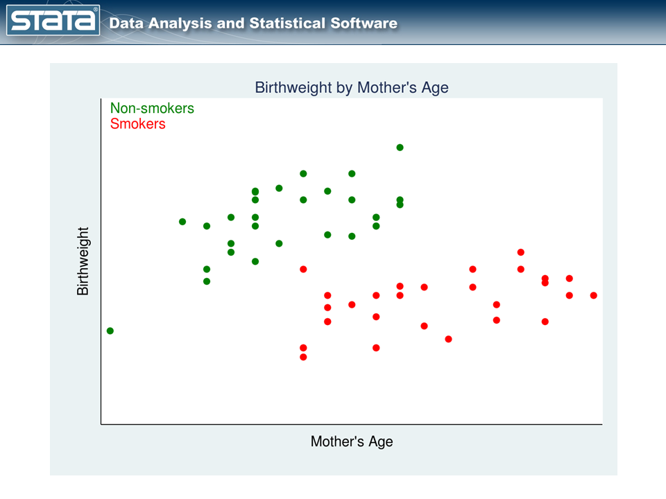
Let’s contemplate an instance. Determine 1 is a scatterplot of observational information much like these utilized by Cattaneo (2010). The therapy variable is the mom’s smoking standing throughout being pregnant, and the end result is the birthweight of her child.
The crimson factors symbolize the moms who smoked throughout being pregnant, whereas the inexperienced factors symbolize the moms who didn’t. The moms themselves selected whether or not to smoke, and that complicates the evaluation.
We can’t estimate the impact of smoking on birthweight by evaluating the imply birthweights of infants of moms who did and didn’t smoke. Why not? Look once more at our graph. Older moms are likely to have heavier infants no matter whether or not they smoked whereas pregnant. In these information, older moms have been additionally extra prone to be people who smoke. Thus, mom’s age is said to each therapy standing and consequence. So how ought to we proceed?
RA: The regression adjustment estimator
RA estimators mannequin the end result to account for the nonrandom therapy project.
We would ask, “How would the outcomes have modified had the moms who smoked chosen to not smoke?” or “How would the outcomes have modified had the moms who didn’t smoke chosen to smoke?”. If we knew the solutions to those counterfactual questions, evaluation could be straightforward: we’d simply subtract the noticed outcomes from the counterfactual outcomes.
The counterfactual outcomes are known as unobserved potential outcomes within the treatment-effects literature. Typically the phrase unobserved is dropped.
We are able to assemble measurements of those unobserved potential outcomes, and our information may appear like this:
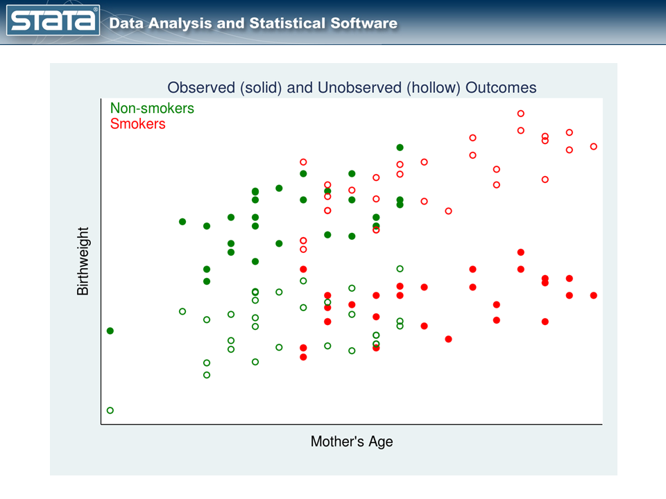
In determine 2, the noticed information are proven utilizing stable factors and the unobserved potential outcomes are proven utilizing hole factors. The hole crimson factors symbolize the potential outcomes for the people who smoke had they not smoked. The hole inexperienced factors symbolize the potential outcomes for the nonsmokers had they smoked.
We are able to estimate the unobserved potential outcomes then by becoming separate linear regression fashions with the noticed information (stable factors) to the 2 therapy teams.
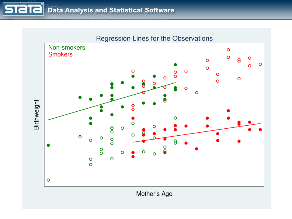
In determine 3, we’ve one regression line for nonsmokers (the inexperienced line) and a separate regression line for people who smoke (the crimson line).
Let’s perceive what the 2 strains imply:
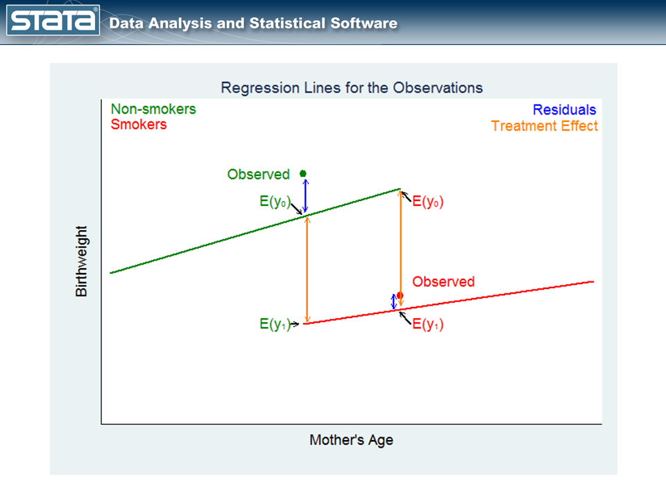
The inexperienced level on the left in determine 4, labeled Noticed, is an commentary for a mom who didn’t smoke. The purpose labeled E(y0) on the inexperienced regression line is the anticipated birthweight of the infant given the mom’s age and that she didn’t smoke. The purpose labeled E(y1) on the crimson regression line is the anticipated birthweight of the infant for a similar mom had she smoked.
The distinction between these expectations estimates the covariate-specific therapy impact for individuals who didn’t get the therapy.
Now, let’s take a look at the opposite counterfactual query.
The crimson level on the best in determine 4, labeled Noticed in crimson, is an commentary for a mom who smoked throughout being pregnant. The factors on the inexperienced and crimson regression strains once more symbolize the anticipated birthweights — the potential outcomes — of the mom’s child underneath the 2 therapy situations.
The distinction between these expectations estimates the covariate-specific therapy impact for individuals who acquired the therapy.
Be aware that we estimate a median therapy impact (ATE), conditional on covariate values, for every topic. Moreover, we estimate this impact for every topic, no matter which therapy was truly acquired. Averages of those results over all the themes within the information estimate the ATE.
We may additionally use determine 4 to encourage a prediction of the end result that every topic would receive for every therapy degree, whatever the therapy recieved. The story is analogous to the one above. Averages of those predictions over all the themes within the information estimate the potential-outcome means (POMs) for every therapy degree.
It’s reassuring that variations within the estimated POMs is similar estimate of the ATE mentioned above.
The ATE on the handled (ATET) is just like the ATE, however it makes use of solely the themes who have been noticed within the therapy group. This method to calculating therapy results is named regression adjustment (RA).
Let’s open a dataset and do that utilizing Stata.
. webuse cattaneo2.dta, clear
(Excerpt from Cattaneo (2010) Journal of Econometrics 155: 138-154)

To estimate the POMs within the two therapy teams, we sort

. teffects ra (bweight mage) (mbsmoke), pomeans
We specify the end result mannequin within the first set of parentheses with the end result variable adopted by its covariates. On this instance, the end result variable is bweight and the one covariate is mage.
We specify the therapy mannequin — merely the therapy variable — within the second set of parentheses. On this instance, we specify solely the therapy variable mbsmoke. We’ll discuss covariates within the subsequent part.
The results of typing the command is
. teffects ra (bweight mage) (mbsmoke), pomeans

Iteration 0:   EE criterion =  7.878e-24
Iteration 1:   EE criterion =  8.468e-26

Remedy-effects estimation                    Variety of obs      =      4642
Estimator      : regression adjustment
Consequence mannequin  : linear
Remedy mannequin: none
------------------------------------------------------------------------------
             |               Strong
     bweight |      Coef.   Std. Err.      z    P>|z|     [95% Conf. Interval]
-------------+----------------------------------------------------------------
POmeans      |
     mbsmoke |
  nonsmoker  |   3409.435   9.294101   366.84   0.000     3391.219    3427.651
     smoker  |   3132.374   20.61936   151.91   0.000     3091.961    3172.787
------------------------------------------------------------------------------
The output experiences that the common birthweight could be 3,132 grams if all moms smoked and three,409 grams if no mom smoked.
We are able to estimate the ATE of smoking on birthweight by subtracting the POMs: 3132.374 – 3409.435 = -277.061. Or we are able to reissue our teffects ra command with the ate possibility and get customary errors and confidence intervals:
. teffects ra (bweight mage) (mbsmoke), ate

Iteration 0:   EE criterion =  7.878e-24
Iteration 1:   EE criterion =  5.185e-26

Remedy-effects estimation                    Variety of obs      =      4642
Estimator      : regression adjustment
Consequence mannequin  : linear
Remedy mannequin: none
-------------------------------------------------------------------------------
              |               Strong
      bweight |      Coef.   Std. Err.      z    P>|z|     [95% Conf. Interval]
--------------+----------------------------------------------------------------
ATE           |
      mbsmoke |
(smoker vs    |
  nonsmoker)  |  -277.0611   22.62844   -12.24   0.000    -321.4121   -232.7102
--------------+----------------------------------------------------------------
POmean        |
      mbsmoke |
   nonsmoker  |   3409.435   9.294101   366.84   0.000     3391.219    3427.651
-------------------------------------------------------------------------------
The output experiences the identical ATE we calculated by hand: -277.061. The ATE is the common of the variations between the birthweights when every mom smokes and the birthweights when no mom smokes.
We are able to additionally estimate the ATET through the use of the teffects ra command with possibility atet, however we is not going to accomplish that right here.
IPW: The inverse chance weighting estimator
RA estimators mannequin the end result to account for the nonrandom therapy project. Some researchers desire to mannequin the therapy project course of and never specify a mannequin for the end result.
We all know that people who smoke are typically older than nonsmokers in our information. We additionally hypothesize that mom’s age straight impacts birthweight. We noticed this in determine 1, which we present once more under.
This determine reveals that therapy project depends upon mom’s age. We wish to have a way of adjusting for this dependence. Particularly, we want we had extra upper-age inexperienced factors and lower-age crimson factors. If we did, the imply birthweight for every group would change. We don’t understand how that will have an effect on the distinction in means, however we do know it will be a greater estimate of the distinction.
To attain an analogous outcome, we’re going to weight people who smoke within the lower-age vary and nonsmokers within the upper-age vary extra closely, and weight people who smoke within the upper-age vary and nonsmokers within the lower-age vary much less closely.
We’ll match a probit or logit mannequin of the shape
Pr(lady smokes) = F(a + b*age)
teffects makes use of logit by default, however we are going to specify the probit possibility for illustration.
As soon as we’ve match that mannequin, we are able to receive the prediction Pr(lady smokes) for every commentary within the information; we’ll name this pi. Then, in making our POMs calculations — which is only a imply calculation — we are going to use these chances to weight the observations. We’ll weight observations on people who smoke by 1/pi in order that weights shall be giant when the chance of being a smoker is small. We’ll weight observations on nonsmokers by 1/(1-pi) in order that weights shall be giant when the chance of being a nonsmoker is small.
That ends in the next graph changing determine 1:
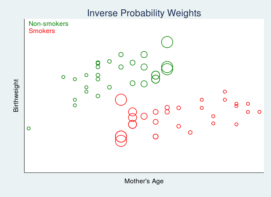
In determine 5, bigger circles point out bigger weights.
To estimate the POMs with this IPW estimator, we are able to sort
. teffects ipw (bweight) (mbsmoke mage, probit), pomeans
The primary set of parentheses specifies the end result mannequin, which is just the end result variable on this case; there are not any covariates. The second set of parentheses specifies the therapy mannequin, which incorporates the end result variable (mbsmoke) adopted by covariates (on this case, simply mage) and the form of mannequin (probit).
The result’s
. teffects ipw (bweight) (mbsmoke mage, probit), pomeans

Iteration 0:   EE criterion =  3.615e-15
Iteration 1:   EE criterion =  4.381e-25

Remedy-effects estimation                    Variety of obs      =      4642
Estimator      : inverse-probability weights
Consequence mannequin  : weighted imply
Remedy mannequin: probit
------------------------------------------------------------------------------
             |               Strong
     bweight |      Coef.   Std. Err.      z    P>|z|     [95% Conf. Interval]
-------------+----------------------------------------------------------------
POmeans      |
     mbsmoke |
  nonsmoker  |   3408.979   9.307838   366.25   0.000     3390.736    3427.222
     smoker  |   3133.479   20.66762   151.61   0.000     3092.971    3173.986
------------------------------------------------------------------------------
Our output experiences that the common birthweight could be 3,133 grams if all of the moms smoked and three,409 grams if not one of the moms smoked.
This time, the ATE is -275.5, and if we typed
. teffects ipw (bweight) (mbsmoke mage, probit), ate
(Output omitted)
we’d be taught that the usual error is 22.68 and the 95% confidence interval is [-319.9,231.0].
Simply as with teffects ra, if we needed ATET, we may specify the teffects ipw command with the atet possibility.
IPWRA: The IPW with regression adjustment estimator
RA estimators mannequin the end result to account for the nonrandom therapy project. IPW estimators mannequin the therapy to account for the nonrandom therapy project. IPWRA estimators mannequin each the end result and the therapy to account for the nonrandom therapy project.
IPWRA makes use of IPW weights to estimate corrected regression coefficients which can be subsequently used to carry out regression adjustment.
The covariates within the consequence mannequin and the therapy mannequin would not have to be the identical, and so they typically should not as a result of the variables that affect a topic’s choice of therapy group are sometimes completely different from the variables related to the end result. The IPWRA estimator has the double-robust property, which signifies that the estimates of the consequences shall be constant if both the therapy mannequin or the end result mannequin — however not each — are misspecified.
Let’s contemplate a state of affairs with extra complicated consequence and therapy fashions however nonetheless utilizing our low-birthweight information.
The result mannequin will embody
- mage: the mom’s age
- prenatal1: an indicator for prenatal go to throughout the first trimester
- mmarried: an indicator for marital standing of the mom
- fbaby: an indicator for being first born
The therapy mannequin will embody
- all of the covariates of the end result mannequin
- mage^2
- medu: years of maternal schooling
We will even specify the aequations choice to report the coefficients of the end result and therapy fashions.
. teffects ipwra (bweight mage prenatal1 mmarried fbaby)                ///
                 (mbsmoke mmarried c.mage##c.mage fbaby medu, probit)   ///
                 , pomeans aequations

Iteration 0:   EE criterion =  1.001e-20
Iteration 1:   EE criterion =  1.134e-25

Remedy-effects estimation                    Variety of obs      =      4642
Estimator      : IPW regression adjustment
Consequence mannequin  : linear
Remedy mannequin: probit
-------------------------------------------------------------------------------
              |               Strong
      bweight |      Coef.   Std. Err.      z    P>|z|     [95% Conf. Interval]
--------------+----------------------------------------------------------------
POmeans       |
      mbsmoke |
   nonsmoker  |   3403.336    9.57126   355.58   0.000     3384.576    3422.095
      smoker  |   3173.369   24.86997   127.60   0.000     3124.624    3222.113
--------------+----------------------------------------------------------------
OME0          |
         mage |   2.893051   2.134788     1.36   0.175    -1.291056    7.077158
    prenatal1 |   67.98549   28.78428     2.36   0.018     11.56933    124.4017
     mmarried |   155.5893   26.46903     5.88   0.000      103.711    207.4677
        fbaby |   -71.9215   20.39317    -3.53   0.000    -111.8914   -31.95162
        _cons |   3194.808   55.04911    58.04   0.000     3086.913    3302.702
--------------+----------------------------------------------------------------
OME1          |
         mage |  -5.068833   5.954425    -0.85   0.395    -16.73929    6.601626
    prenatal1 |   34.76923   43.18534     0.81   0.421    -49.87248    119.4109
     mmarried |   124.0941   40.29775     3.08   0.002     45.11193    203.0762
        fbaby |   39.89692   56.82072     0.70   0.483    -71.46966    151.2635
        _cons |   3175.551   153.8312    20.64   0.000     2874.047    3477.054
--------------+----------------------------------------------------------------
TME1          |
     mmarried |  -.6484821   .0554173   -11.70   0.000     -.757098   -.5398663
         mage |   .1744327   .0363718     4.80   0.000     .1031452    .2457202
              |
c.mage#c.mage |  -.0032559   .0006678    -4.88   0.000    -.0045647   -.0019471
              |
        fbaby |  -.2175962   .0495604    -4.39   0.000    -.3147328   -.1204595
         medu |  -.0863631   .0100148    -8.62   0.000    -.1059917   -.0667345
        _cons |  -1.558255   .4639691    -3.36   0.001    -2.467618   -.6488926
-------------------------------------------------------------------------------
The POmeans part of the output shows the POMs for the 2 therapy teams. The ATE is now calculated to be 3173.369 – 3403.336 = -229.967.
The OME0 and OME1 sections show the RA coefficients for the untreated and handled teams, respectively.
The TME1 part of the output shows the coefficients for the probit therapy mannequin.
Simply as within the two earlier instances, if we needed the ATE with customary errors, and many others., we’d specify the ate possibility. If we needed ATET, we’d specify the atet possibility.
AIPW: The augmented IPW estimator
IPWRA estimators mannequin each the end result and the therapy to account for the nonrandom therapy project. So do AIPW estimators.
The AIPW estimator provides a bias-correction time period to the IPW estimator. If the therapy mannequin is accurately specified, the bias-correction time period is 0 and the mannequin is lowered to the IPW estimator. If the therapy mannequin is misspecified however the consequence mannequin is accurately specified, the bias-correction time period corrects the estimator. Thus, the bias-correction time period offers the AIPW estimator the identical double-robust property because the IPWRA estimator.
The syntax and output for the AIPW estimator is nearly similar to that for the IPWRA estimator.
. teffects aipw (bweight mage prenatal1 mmarried fbaby)                 ///
                (mbsmoke mmarried c.mage##c.mage fbaby medu, probit)    ///
                , pomeans aequations

Iteration 0:   EE criterion =  4.632e-21
Iteration 1:   EE criterion =  5.810e-26

Remedy-effects estimation                    Variety of obs      =      4642
Estimator      : augmented IPW
Consequence mannequin  : linear by ML
Remedy mannequin: probit
-------------------------------------------------------------------------------
              |               Strong
      bweight |      Coef.   Std. Err.      z    P>|z|     [95% Conf. Interval]
--------------+----------------------------------------------------------------
POmeans       |
      mbsmoke |
   nonsmoker  |   3403.355   9.568472   355.68   0.000     3384.601    3422.109
      smoker  |   3172.366   24.42456   129.88   0.000     3124.495    3220.237
--------------+----------------------------------------------------------------
OME0          |
         mage |   2.546828   2.084324     1.22   0.222    -1.538373    6.632028
    prenatal1 |   64.40859   27.52699     2.34   0.019     10.45669    118.3605
     mmarried |   160.9513    26.6162     6.05   0.000     108.7845    213.1181
        fbaby |   -71.3286   19.64701    -3.63   0.000     -109.836   -32.82117
        _cons |   3202.746   54.01082    59.30   0.000     3096.886    3308.605
--------------+----------------------------------------------------------------
OME1          |
         mage |  -7.370881    4.21817    -1.75   0.081    -15.63834    .8965804
    prenatal1 |   25.11133   40.37541     0.62   0.534    -54.02302    104.2457
     mmarried |   133.6617   40.86443     3.27   0.001      53.5689    213.7545
        fbaby |   41.43991   39.70712     1.04   0.297    -36.38461    119.2644
        _cons |   3227.169   104.4059    30.91   0.000     3022.537    3431.801
--------------+----------------------------------------------------------------
TME1          |
     mmarried |  -.6484821   .0554173   -11.70   0.000     -.757098   -.5398663
         mage |   .1744327   .0363718     4.80   0.000     .1031452    .2457202
              |
c.mage#c.mage |  -.0032559   .0006678    -4.88   0.000    -.0045647   -.0019471
              |
        fbaby |  -.2175962   .0495604    -4.39   0.000    -.3147328   -.1204595
         medu |  -.0863631   .0100148    -8.62   0.000    -.1059917   -.0667345
        _cons |  -1.558255   .4639691    -3.36   0.001    -2.467618   -.6488926
-------------------------------------------------------------------------------
The ATE is 3172.366 – 3403.355 = -230.989.
Ultimate ideas
The instance above used a steady consequence: birthweight. teffects will also be used with binary, depend, and nonnegative steady outcomes.
The estimators additionally permit a number of therapy classes.
A complete guide is dedicated to the treatment-effects options in Stata 13, and it features a fundamental introduction, superior dialogue, and labored examples. If you want to be taught extra, you’ll be able to obtain the [TE] Remedy-effects Reference Guide from the Stata web site.
Extra to come back
Subsequent time, partially 2, we are going to cowl the matching estimators.
Reference
Cattaneo, M. D. 2010. Environment friendly semiparametric estimation of multi-valued therapy results underneath ignorability. Journal of Econometrics 155: 138–154.