Effectivity comparisons by Monte Carlo simulation

Overview

On this submit, I present find out how to use Monte Carlo simulations to check the effectivity of various estimators. I additionally illustrate what we imply by effectivity when discussing statistical estimators.

I wrote this submit to proceed a dialog with my buddy who doubted the usefulness of the pattern common as an estimator for the imply when the data-generating course of (DGP) is a (chi^2) distribution with (1) diploma of freedom, denoted by a (chi^2(1)) distribution. The pattern common is a fantastic estimator, despite the fact that it isn’t probably the most environment friendly estimator for the imply. (Some researchers choose to estimate the median as an alternative of the imply for DGPs that generate outliers. I’ll deal with the trade-offs between these parameters in a future submit. For now, I need to follow estimating the imply.)

On this submit, I additionally need to illustrate that Monte Carlo simulations will help clarify summary statistical ideas. I present find out how to use a Monte Carlo simulation for example the which means of an summary statistical idea. (In case you are new to Monte Carlo simulations in Stata, you may need to see Monte Carlo simulations utilizing Stata.)

Constant estimator A is claimed to be extra asymptotically environment friendly than constant estimator B if A has a smaller asymptotic variance than B; see Wooldridge (2010, sec. 14.4.2) for an particularly helpful dialogue. Theoretical comparisons can typically confirm that A is extra environment friendly than B, however the magnitude of the distinction isn’t recognized. Comparisons of Monte Carlo simulation estimates of the variances of estimators A and B give each signal and magnitude for particular DGPs and pattern sizes.

The pattern common versus most chance

Many books talk about the situations beneath which the utmost chance (ML) estimator is the environment friendly estimator relative to different estimators; see Wooldridge (2010, sec. 14.4.2) for an accessible introduction to the fashionable strategy. Right here I evaluate the ML estimator with the pattern common for the imply when the DGP is a (chi^2(1)) distribution.

Instance 1 under accommodates the instructions I used. For an introduction to Monte Carlo simulations see Monte Carlo simulations utilizing Stata, and for an introduction to utilizing mlexp to estimate the parameter of a (chi^2) distribution see Most chance estimation by mlexp: A chi-squared instance. Briefly, the instructions do the next (5,000) occasions:

1. Draw a pattern of 500 observations from a (chi^2(1)) distribution.
2. Estimate the imply of every pattern by the pattern common, and retailer this estimate in m_a within the dataset efcomp.dta.
3. Estimate the imply of every pattern by ML, and retailer this estimate in m_ml within the dataset efcomp.dta.

Instance 1: The distributions of the pattern common and the ML estimators

. clear all
. set seed 12345
. postfile sim  mu_a mu_ml utilizing efcomp, exchange
. forvalues i = 1/5000 {
  2.     quietly drop _all
  3.     quietly set obs 500
  4.     quietly generate double y = rchi2(1)
  5.     quietly imply y 
  6.     native mu_a         =  _b[y]
  7.     quietly mlexp (ln(chi2den({d=1},y)))
  8.     native mu_ml   =  _b[d:_cons]
  9.     submit sim (`mu_a') (`mu_ml') 
 10. }
. postclose sim
. use efcomp, clear 
. summarize

    Variable |        Obs        Imply    Std. Dev.       Min        Max
-------------+---------------------------------------------------------
        mu_a |      5,000    .9989277    .0620524   .7792076   1.232033
       mu_ml |      5,000    1.000988    .0401992   .8660786   1.161492

The imply of the (5,000) pattern common estimates and the imply of the (5,000) ML estimates are every near the true worth of (1.0). The usual deviation of the (5,000) pattern common estimates is (0.062), and it approximates the usual deviation of the sampling distribution of the pattern common for this DGP and pattern measurement. Equally, the usual deviation of the (5,000) ML estimates is (0.040), and it approximates the usual deviation of the sampling distribution of the ML estimator for this DGP and pattern measurement.

We conclude that the ML estimator has a decrease variance than the pattern common for this DGP and this pattern measurement, as a result of (0.040) is smaller than (0.062).

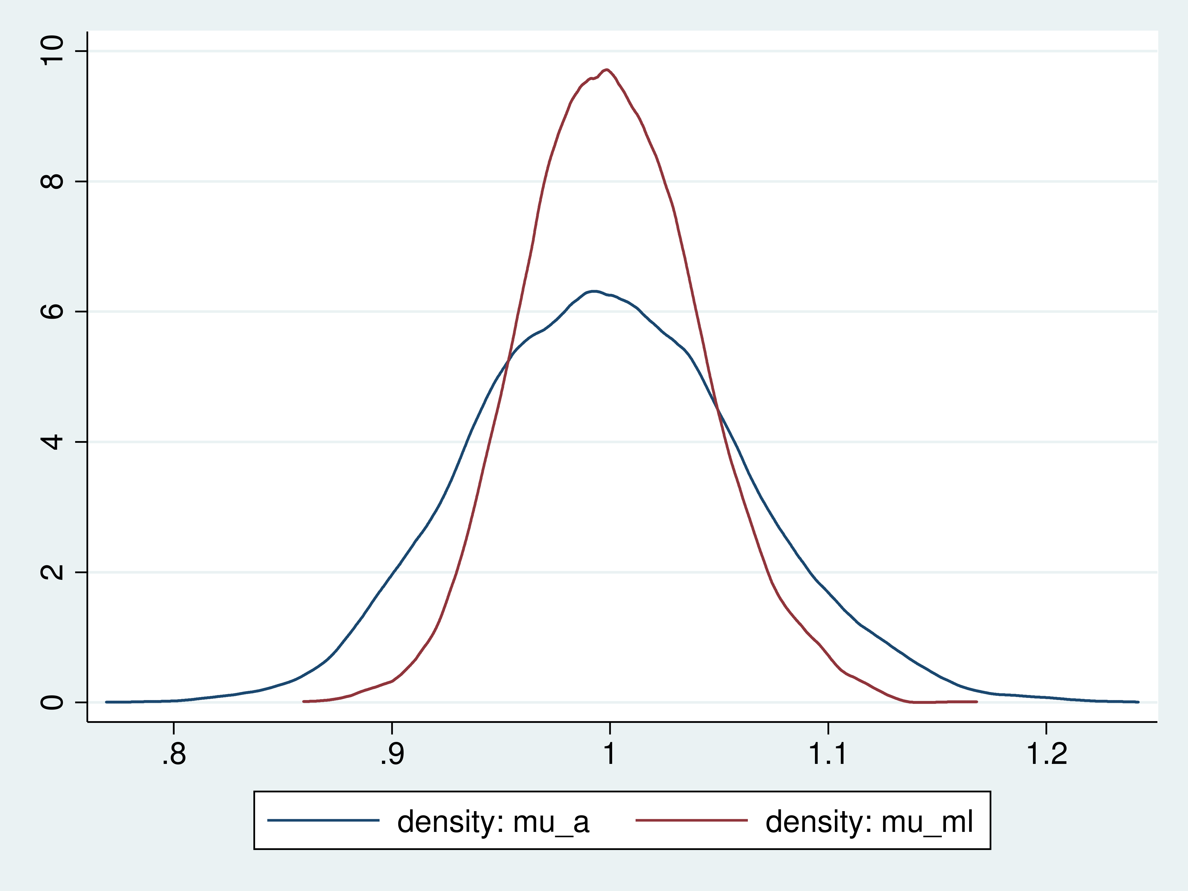
To get an image of this distinction, we plot the density of the pattern common and the density of the ML estimator. (Every of those densities is estimated from (5,000) observations, however estimation error may be ignored as a result of extra knowledge wouldn’t change the important thing outcomes.)

Instance 2: Plotting the densities of the estimators

. kdensity mu_a,   n(5000) generate(x_a   den_a)   nograph

. kdensity mu_ml,  n(5000) generate(x_ml  den_ml)  nograph

. twoway (line den_a x_a) (line den_ml x_ml)

Densities of the pattern common and ML estimators

The plots present that the ML estimator is extra tightly distributed across the true worth than the pattern common.

That the ML estimator is extra tightly distributed across the true worth than the pattern common is what it means for one constant estimator to be extra environment friendly than one other.

Completed and undone

I used Monte Carlo simulation for example what it means for one estimator to be extra environment friendly than one other. Specifically, we noticed that the ML estimator is extra environment friendly than the pattern common for the imply of a (chi^2(1)) distribution.

Many different estimators fall between these two estimators in an effectivity rating. Generalized technique of moments estimators and a few quasi-maximum chance estimators come to thoughts and is perhaps value including to those simulations.

Reference

Wooldridge, J. M. 2010. Econometric Evaluation of Cross Part and Panel Information. 2nd ed. Cambridge, Massachusetts: MIT Press.