

Introduction
Machine studying strategies, reminiscent of ensemble resolution timber, are broadly used to foretell outcomes primarily based on information. Nevertheless, these strategies typically give attention to offering level predictions, which limits their potential to quantify prediction uncertainty. In lots of functions, reminiscent of healthcare and finance, the aim just isn’t solely to foretell precisely but in addition to evaluate the reliability of these predictions. Prediction intervals, which offer decrease and higher bounds such that the true response lies inside them with excessive chance, are a dependable instrument for quantifying prediction accuracy. A great prediction interval ought to meet a number of standards: it ought to provide legitimate protection (outlined under) with out counting on robust distributional assumptions, be informative by being as slim as attainable for every remark, and be adaptive—present wider intervals for observations which might be “troublesome” to foretell and narrower intervals for “straightforward” ones.
You might ponder whether it’s attainable to assemble a statistically legitimate prediction interval utilizing any machine studying methodology, with none distributional assumption reminiscent of Gaussianity, whereas the above standards are happy. Wait and see.
On this submit, I exhibit the way to use Stata’s h2oml suite of instructions to assemble predictive intervals by utilizing the conformalized quantile regression (CQR) strategy, launched in Romano, Patterson, and Candes (2019). The construction of the submit is as follows: First, I present a short introduction to conformal prediction, with a give attention to CQR, after which I present the way to assemble predictive intervals in Stata by utilizing gradient boosting regressions.
Conformal prediction
Conformal prediction (Papadopoulos et al. 2002; Vovk, Gammerman, and Shafer 2005; Lei et al. 2018; Angelopoulos and Bates 2023), also referred to as conformal inference, is a basic methodology designed to enrich any machine studying prediction by offering prediction intervals with assured distribution-free statistical protection. At a conceptual degree, conformal prediction begins with a pretrained machine studying mannequin (for instance, a gradient boosting machine) skilled on exchangeable or impartial and identically distributed information. It then makes use of held-out validation information from the identical data-generating distribution, known as calibration information, to outline a rating operate (S(hat y, y)). This operate assigns bigger scores when the discrepancy between the anticipated worth (hat y) and the true response (y) is larger. These scores are subsequently used to assemble prediction intervals for brand new, unseen observations ({bf X}_{textual content{new}}), the place ({bf X}_{textual content{new}}) is a random vector of predictors.
It may be proven that conformal prediction (mathcal{C}({bf X}_{textual content{new}})) gives legitimate prediction interval protection (Lei et al. 2018; Angelopoulos and Bates 2023) within the sense that
[
P{Y_{text{new}} in mathcal{C}({bf X}_{text{new}})} geq 1 – alpha tag{1}label{eq1}
]
the place (alpha in (0,1)) is a user-defined miscoverage or error fee. This property is named marginal protection, as a result of the chance is averaged over the randomness of calibration and unseen or testing information.
Though the conformal prediction strategy ensures legitimate protection eqref{eq1} with minimal distributional assumptions and for any machine studying methodology, our focus right here is on CQR (Romano, Patterson, and Candes 2019). It is without doubt one of the most generally used and really helpful approaches to assemble prediction intervals (Romano, Patterson, and Candes 2019; Angelopoulos and Bates 2023).
CQR
The publicity on this part intently follows Romano, Patterson, and Candes (2019) and Angelopoulos and Bates (2023). Take into account a quantile regression that estimates a conditional quantile operate (q_{alpha}(cdot)) of (Y_{textual content{new}}) given ({bf X}_{textual content{new}} = {bf x}) for every attainable realization of ({bf x}). We are able to use any quantile regression estimation methodology, reminiscent of gradient boosting machine with quantile or “pinball” loss to acquire (widehat q_{alpha}(cdot)). By definition, (Y_{textual content{new}}|{bf X}_{textual content{new}} = {bf x}) is under (q_{alpha/2}({bf x})) with chance (alpha/2) and above (q_{1 – alpha/2}({bf x})) with chance (alpha/2), so the estimated prediction interval ([widehat q_{alpha/2}(cdot), widehat q_{1 – alpha/2}(cdot)]) ought to have roughly (1-alpha)% protection. Sadly, as a result of the estimated quantiles may be inaccurate, such protection just isn’t assured. Thus, we have to conformalize them to have a legitimate protection eqref{eq1}. CQR steps may be summarized as follows:
- Step 1. Break up information (mathcal{D}) right into a coaching (mathcal{D}_1) and calibration (mathcal{D}_2), and let (mathcal{D}_3) be the brand new, unseen testing information.
- Step 2. Use (mathcal{D}_1) to coach any quantile regression estimation methodology (f) to estimate two conditional quantile features (hat q_{alpha_1}(cdot)) and (hat q_{alpha_2}(cdot)), for (alpha_1 = alpha/2) and (alpha_2 = 1 – alpha/2), respectively. For instance, when the miscoverage fee (alpha = 0.1), we acquire (hat q_{0.05}(cdot)) and (hat q_{0.95}(cdot)).
- Step 3. Use calibration information (mathcal{D}_2) to compute conformity scores (S_i), for every (i in mathcal{D}_2), that quantify the error made by the interval ([hat q_{alpha_1}({bf x}), hat q_{alpha_2}({bf x})]).
[
S_i = max {hat q_{alpha_1}({bf x}_i) – Y_i, Y_i – hat q_{alpha_2}({bf x}_i)}
] - Step 4. Given new unseen information ({bf X}_{textual content{new}} subset mathcal{D}_3), assemble the prediction interval for (Y_{textual content{new}}),
[
mathcal{C}({bf X}_{text{new}}) = Big[hat q_{alpha_1}({bf X}_{text{new}}) – q_{1 – alpha}(S_i, mathcal{D}_2), hat q_{alpha_2}({bf X}_{text{new}}) + q_{1 – alpha}(S_i, mathcal{D}_2)Big]
]
the place the empirical quantile of conformity scores
[ label{eq:empquantile}
q_{1 – alpha}(S_i, mathcal{D}_2) = frac{lceil (|mathcal{D}_2|+1)(1 – alpha) rceil}{|mathcal{D}_2|} tag{2}
]
and (|mathcal{D}_2|) is the variety of observations of the calibration information and (lceil cdot rceil) is the ceiling operate.
The instinct behind the conformity rating, computed in step 3, is the next:
- If (Y_{textual content{new}} < q_{alpha_1}({bf X}_{textual content{new}})) or (Y_{textual content{new}} > q_{alpha_2}({bf X}_{textual content{new}})), the scores given by (S_i = |Y_{textual content{new}} – q_{alpha_1}({bf X}_{textual content{new}})|) or (S_i = |Y_{textual content{new}} – q_{alpha_2}({bf X}_{textual content{new}})|) symbolize the magnitude of the error incurred by this error.
- Then again, if (q_{alpha_1}({bf X}_{textual content{new}}) leq Y_{textual content{new}} leq q_{alpha_2}({bf X}_{textual content{new}})), the computed rating is at all times nonpositive.
This fashion, the conformity rating accounts for each undercoverage and overcoverage.
Romano, Patterson, and Candes (2019) confirmed that below the exchangeability assumption, steps 1–4 assure the legitimate marginal protection eqref{eq1}.
Implementation in Stata
On this part, we use the h2oml suite of instructions in Stata to assemble predictive intervals utilizing conformalized gradient boosting quantile regression. H2O is a scalable and distributed machine studying and predictive analytics platform that permits us to carry out information evaluation and machine studying. For particulars, see the Stata 19 Machine Studying in Stata Utilizing H2O: Ensemble Determination Bushes Reference Handbook.
We think about the Ames housing dataset (De Cock 2011), ameshouses.dta, additionally utilized in a Kaggle competitors, which describes residential homes offered in Ames, Iowa, between 2006 and 2010. It comprises about 80 housing (and associated) traits, reminiscent of house dimension, facilities, and placement. This dataset is usually used for constructing predictive fashions for house sale worth, saleprice. Earlier than placing the dataset into an H2O body, we carry out some information manipulation in Stata. As a result of saleprice is right-skewed (for instance, sort histogram saleprice), we use its log. We additionally generate a variable, houseage, that calculates the age of the home on the time of a gross sales transaction.
. webuse ameshouses

. generate logsaleprice = log(saleprice)

. generate houseage = yrsold - yearbuilt

. drop saleprice yrsold yearbuilt
Subsequent, we initialize a cluster and put the information into an H2O body. Then, to carry out step 1, let’s cut up the information into coaching (50%), calibration (40%), and testing (10%) frames, the place the testing body serves as a proxy for brand new, unseen information.
. h2o init
(output omitted)

. _h2oframe put, into(home)

Progress (%): 0 100

. _h2oframe cut up home, into(prepare calib check) cut up(0.5 0.4 0.1)
> rseed(1)

. _h2oframe change prepare
Our aim is to assemble a predictive interval with 90% protection. We outline three native macros in Stata to retailer the miscoverage fee (alpha = 1- 0.9 = 0.1) and decrease and higher bounds, (0.05) and (0.95), respectively. Let’s additionally create a worldwide macro, predictors, that comprises the names of our predictors.
. native alpha = 0.1

. native decrease = 0.05

. native higher = 0.95

. international predictors overallqual grlivarea exterqual houseage garagecars
> totalbsmtsf stflrsf garagearea kitchenqual bsmtqual
We carry out step 2 by pretraining gradient boosting quantile regression by utilizing the h2oml gbregress command with the loss(quantile) possibility. For illustration, I tune solely the variety of timber (ntrees()) and maximum-depth (maxdepth()) hyperparameters, and retailer the estimation outcomes by utilizing the h2omlest retailer command.
. h2oml gbregress logsaleprice $predictors, h2orseed(19) cv(3, modulo)
> loss(quantile, alpha(`decrease')) ntrees(20(20)80) maxdepth(6(2)12)
> tune(grid(cartesian))

Progress (%): 0 100

Gradient boosting regression utilizing H2O

Response: logsaleprice
Loss:     Quantile .05
Body:                                 Variety of observations:
  Coaching: prepare                                 Coaching =    737
                                          Cross-validation =    737
Cross-validation: Modulo               Variety of folds     =      3

Tuning data for hyperparameters

Methodology: Cartesian
Metric: Deviance

-------------------------------------------------------------------
                 |                      Grid values
 Hyperparameters |         Minimal          Most        Chosen
-----------------+-------------------------------------------------
 Variety of timber |              20               80              40
 Max. tree depth |               6               12               8
-------------------------------------------------------------------

Mannequin parameters

Variety of timber      =  40             Studying fee       =     .1
              precise =  40             Studying fee decay =      1
Tree depth:                            Pred. sampling fee =      1
           Enter max =   8             Sampling fee       =      1
                 min =   6             No. of bins cat.    =  1,024
                 avg = 7.5             No. of bins root    =  1,024
                 max =   8             No. of bins cont.   =     20
Min. obs. leaf cut up =  10             Min. cut up thresh.  = .00001
Metric abstract
-----------------------------------
           |                 Cross-
    Metric |   Coaching  validation
-----------+-----------------------
  Deviance |   .0138451    .0259728
       MSE |   .1168036    .1325075
      RMSE |   .3417654    .3640158
     RMSLE |   .0259833    .0278047
       MAE |   .2636412    .2926809
 R-squared |   .3117896    .2192615
-----------------------------------

. h2omlest retailer q_lower
The very best-selected mannequin has 40 timber and a most tree depth of 8. I exploit this mannequin to acquire predicted decrease quantiles on the calibration dataset by utilizing the h2omlpredict command with the body() possibility. We’ll use these predicted values to compute conformity scores in step 3.
. h2omlpredict q_lower, body(calib)

Progress (%): 0 100
For simplicity, I exploit the above hyperparameters to run gradient boosting quantile regression for the higher quantile. In follow, we have to tune hyperparameters for this mannequin as effectively. As earlier than, I predict the higher quantiles on the calibration dataset and retailer the mannequin.
. h2oml gbregress logsaleprice $predictors, h2orseed(19) cv(3, modulo)
> loss(quantile, alpha(`higher')) ntrees(40) maxdepth(8)

Progress (%): 0 1.2 100

Gradient boosting regression utilizing H2O

Response: logsaleprice
Loss:     Quantile .95
Body:                                 Variety of observations:
  Coaching: prepare                                 Coaching =    737
                                          Cross-validation =    737
Cross-validation: Modulo               Variety of folds     =      3

Mannequin parameters

Variety of timber      =  40             Studying fee       =     .1
              precise =  40             Studying fee decay =      1
Tree depth:                            Pred. sampling fee =      1
           Enter max =   8             Sampling fee       =      1
                 min =   5             No. of bins cat.    =  1,024
                 avg = 7.2             No. of bins root    =  1,024
                 max =   8             No. of bins cont.   =     20
Min. obs. leaf cut up =  10             Min. cut up thresh.  = .00001

Metric abstract
-----------------------------------
           |                 Cross-
    Metric |   Coaching  validation
-----------+-----------------------
  Deviance |   .0132103    .0218716
       MSE |   .1190689    .1365112
      RMSE |   .3450637    .3694742
     RMSLE |   .0268811    .0287084
       MAE |   .2567844    .2841911
 R-squared |   .2984421    .1956718
-----------------------------------

. h2omlest retailer q_upper

. h2omlpredict q_upper, body(calib)

Progress (%): 0 100
To compute conformity scores as in step 3, let’s use the _h2oframe get command to load the estimated quantiles and the logarithm of the gross sales worth from the calibration body calib into Stata. As a result of the information in Stata’s reminiscence have been modified, I additionally use the clear possibility.
. _h2oframe get logsaleprice q_lower q_upper utilizing calib, clear
Then, we use these variables to generate a brand new variable, conf_scores, that comprises the computed conformity scores.
. generate double conf_scores =
> max(q_lower - logsaleprice, logsaleprice - q_upper)
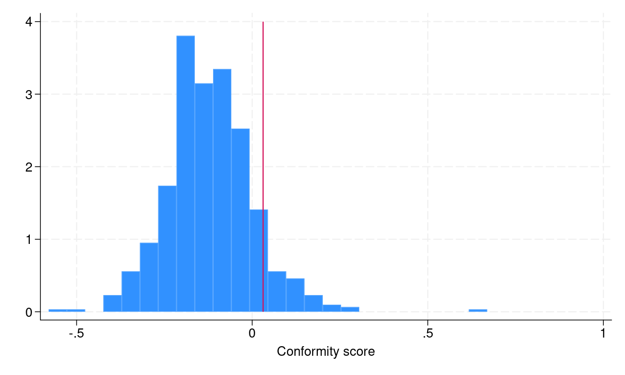
To assemble conformalized prediction intervals from step 4, we have to compute empirical quantiles eqref{eq:empquantile}, which may be executed in Stata by utilizing the _pctile command. Determine 1a exhibits the distribution of conformity scores, and the crimson vertical line signifies the empirical quantile eqref{eq:empquantile}, which is the same as 0.031.
. native emp_quantile = ceil((1 - 0.1) * (_N + 1))/ _N * 100

. _pctile conf_score, percentiles(`emp_quantile')

. native q = r(r1)

. di `q'
.03104496
Subsequent, I restore each fashions that estimated decrease and higher quantiles and procure their predictions on the testing body check.
. h2omlest restore q_lower
(outcomes q_lower are energetic now)

. h2omlpredict q_lower, body(check)

Progress (%): 0 100

. h2omlest restore q_upper
(outcomes q_upper are energetic now)

. h2omlpredict q_upper, body(check)

Progress (%): 0 100
I then load these predictions from the testing body into Stata and generate decrease and higher bounds for prediction intervals. As well as, I additionally load the logsaleprice and houseage variables. We’ll use these variables for illustration functions.
. _h2oframe get logsaleprice houseage q_lower q_upper utilizing check, clear

. generate double conf_lower = q_lower - `q'

. generate double conf_upper = q_upper + `q'
Determine 1b shows the prediction intervals for every remark within the testing body. We are able to see that the computed interval is adaptive, that means for “troublesome” observations, for instance, outliers, the interval is vast and vice versa.
|
(a) Histogram of conformity scores |
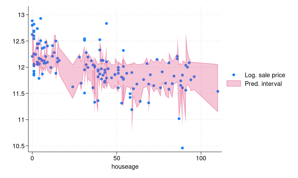 (b) Prediction intervals for the testing dataset |
|
Determine 1: (a) Histogram of conformity scores (b) CQR-based prediction intervals for the testing dataset |
|
Under, I record a small pattern of the prediction intervals and the true log of sale worth response.
. record logsaleprice conf_lower conf_upper in 1/10

     +----------------------------------+
     | logsal~e   conf_lo~r   conf_up~r |
     |----------------------------------|
  1. | 11.67844   11.470275   12.052485 |
  2. |  12.6925   12.002838   12.773621 |
  3. | 11.31447   11.332932   12.058372 |
  4. | 11.64833   11.527202   12.099679 |
  5. | 12.10349   11.640463   12.401743 |
     |----------------------------------|
  6. |  11.8494   11.621721   12.231588 |
  7. |  11.8838   11.631179   12.045645 |
  8. | 12.06681   11.931026   12.204194 |
  9. | 12.12811   11.852887   12.375453 |
 10. | 11.65269   11.569664   12.066292 |
     +----------------------------------+
For 9 out of 10 observations, the responses belong to the respective predictive intervals. We are able to compute the precise common protection of the interval within the testing body, which I do subsequent by producing a brand new variable, in_interval, that signifies whether or not the response logsaleprice is within the prediction interval.
. generate byte in_interval = 0

. substitute in_interval = 1 if inrange(logsaleprice, conf_lower, conf_upper)
(124 actual adjustments made)

. summarize in_interval, meanonly

. native avg_coverage = r(imply)

. di `avg_coverage' * 100
90.510949
We are able to see that the precise common protection is 90.5%.
References
Angelopoulos, A. N., and S. Bates. 2023. Conformal prediction: A delicate introduction. Foundations and Traits in Machine Studying 16: 494–591. https://doi.org/10.1561/2200000101.
De Cock, D. 2011. Ames, Iowa: Different to the Boston housing information as an finish of semester regression mission. Journal of Statistics Training 19: 3. https://doi.org/10.1080/10691898.2011.11889627.
Lei, J., M. G’Promote, A. Rinaldo, R. J. Tibshirani, and L. Wasserman. 2018. Distribution-free predictive inference for regression. Journal of the American Statistical Affiliation 113: 1094–1111. https://doi.org/10.1080/01621459.2017.1307116.
Papadopoulos, H., Okay. Proedrou, V. Vovk, and A. Gammerman. 2002. “Inductive confidence machines for regression”. In Machine Studying: ECML 2002. Lecture Notes in Pc Science, edited by T. Elomaa, H. Mannila, H. Toivonen, vol. 2430: 345–356. Berlin: Springer. https://doi.org/10.1007/3-540-36755-1_29.
Romano, Y., E. Patterson, and E. Candes. 2019. “Conformalized quantile regression”. In Advances in Neural Data Processing Programs, edited by H. Wallach, H. Larochelle, A. Beygelzimer, F. d’Alché-Buc, E. Fox, and R. Garnett, vol. 32. Crimson Hook, NY: Curran Associates, Inc. https://proceedings.neurips.cc/paper_files/paper/2019/file/5103c3584b063c431bd1268e9b5e76fb-Paper.pdf.
Vovk, V., A. Gammerman, and G. Shafer. 2005. Algorithmic Studying in a Random World. New York: Springer. https://doi.org/10.1007/b106715.