
: A easy instance")
(newcommand{Eb}{{bf E}})This publish was written collectively with Enrique Pinzon, Senior Econometrician, StataCorp.
The generalized technique of moments (GMM) is a technique for setting up estimators, analogous to most chance (ML). GMM makes use of assumptions about particular moments of the random variables as an alternative of assumptions about the whole distribution, which makes GMM extra sturdy than ML, at the price of some effectivity. The assumptions are referred to as second circumstances.
GMM generalizes the strategy of moments (MM) by permitting the variety of second circumstances to be better than the variety of parameters. Utilizing these further second circumstances makes GMM extra environment friendly than MM. When there are extra second circumstances than parameters, the estimator is claimed to be overidentified. GMM can effectively mix the second circumstances when the estimator is overidentified.
We illustrate these factors by estimating the imply of a (chi^2(1)) by MM, ML, a easy GMM estimator, and an environment friendly GMM estimator. This instance builds on Effectivity comparisons by Monte Carlo simulation and is comparable in spirit to the instance in Wooldridge (2001).
GMM weights and effectivity
GMM builds on the concepts of anticipated values and pattern averages. Second circumstances are anticipated values that specify the mannequin parameters by way of the true moments. The pattern second circumstances are the pattern equivalents to the second circumstances. GMM finds the parameter values which can be closest to satisfying the pattern second circumstances.
The imply of a (chi^2) random variable with (d) diploma of freedom is (d), and its variance is (2nd). Two second circumstances for the imply are thus
[begin{eqnarray*}
Ebleft[Y – d right]&=& 0
Ebleft[(Y – d )^2 – 2d right]&=& 0
finish{eqnarray*}]
The pattern second equivalents are
[begin{eqnarray}
1/Nsum_{i=1}^N (y_i – widehat{d} )&=& 0 tag{1}
1/Nsum_{i=1}^Nleft[(y_i – widehat{d} )^2 – 2widehat{d}right] &=& 0 tag{2}
finish{eqnarray}]
We might use both pattern second situation (1) or pattern second situation (2) to estimate (d). In truth, beneath we use each and present that (1) gives a way more environment friendly estimator.
Once we use each (1) and (2), there are two pattern second circumstances and just one parameter, so we can not resolve this method of equations. GMM finds the parameters that get as shut as doable to fixing weighted pattern second circumstances.
Uniform weights and optimum weights are two methods of weighting the pattern second circumstances. The uniform weights use an identification matrix to weight the second circumstances. The optimum weights use the inverse of the covariance matrix of the second circumstances.
We start by drawing a pattern of a dimension 500 and use gmm to estimate the parameters utilizing pattern second situation (1), which we illustrate is the pattern because the pattern common.
. drop _all

. set obs 500
variety of observations (_N) was 0, now 500

. set seed 12345

. generate double y = rchi2(1)

. gmm (y - {d})  , devices( ) onestep

Step 1
Iteration 0:   GMM criterion Q(b) =  .82949186
Iteration 1:   GMM criterion Q(b) =  1.262e-32
Iteration 2:   GMM criterion Q(b) =  9.545e-35

notice: mannequin is precisely recognized

GMM estimation

Variety of parameters =   1
Variety of moments    =   1
Preliminary weight matrix: Unadjusted                 Variety of obs   =        500

------------------------------------------------------------------------------
             |               Sturdy
             |      Coef.   Std. Err.      z    P>|z|     [95% Conf. Interval]
-------------+----------------------------------------------------------------
          /d |   .9107644   .0548098    16.62   0.000     .8033392     1.01819
------------------------------------------------------------------------------
Devices for equation 1: _cons

. imply y

Imply estimation                   Variety of obs   =        500

--------------------------------------------------------------
             |       Imply   Std. Err.     [95% Conf. Interval]
-------------+------------------------------------------------
           y |   .9107644   .0548647      .8029702    1.018559
--------------------------------------------------------------
The pattern second situation is the product of an observation-level error operate that’s specified contained in the parentheses and an instrument, which is a vector of ones on this case. The parameter (d) is enclosed in curly braces {}. We specify the onestep choice as a result of the variety of parameters is similar because the variety of second circumstances, which is to say that the estimator is precisely recognized. When it’s, every pattern second situation might be solved precisely, and there are not any effectivity features in optimally weighting the second circumstances.
We now illustrate that we might use the pattern second situation obtained from the variance to estimate (d).
. gmm ((y-{d})^2 - 2*{d})  , devices( ) onestep

Step 1
Iteration 0:   GMM criterion Q(b) =  5.4361161
Iteration 1:   GMM criterion Q(b) =  .02909692
Iteration 2:   GMM criterion Q(b) =  .00004009
Iteration 3:   GMM criterion Q(b) =  5.714e-11
Iteration 4:   GMM criterion Q(b) =  1.172e-22

notice: mannequin is precisely recognized

GMM estimation

Variety of parameters =   1
Variety of moments    =   1
Preliminary weight matrix: Unadjusted                 Variety of obs   =        500

------------------------------------------------------------------------------
             |               Sturdy
             |      Coef.   Std. Err.      z    P>|z|     [95% Conf. Interval]
-------------+----------------------------------------------------------------
          /d |   .7620814   .1156756     6.59   0.000     .5353613    .9888015
------------------------------------------------------------------------------
Devices for equation 1: _cons
Whereas we can not say something definitive from just one draw, we notice that this estimate is farther from the reality and that the usual error is far bigger than these based mostly on the pattern common.
Now, we use gmm to estimate the parameters utilizing uniform weights.
. matrix I = I(2)

. gmm ( y - {d}) ( (y-{d})^2 - 2*{d})  , devices( ) winitial(I) onestep

Step 1
Iteration 0:   GMM criterion Q(b) =   6.265608
Iteration 1:   GMM criterion Q(b) =  .05343812
Iteration 2:   GMM criterion Q(b) =  .01852592
Iteration 3:   GMM criterion Q(b) =   .0185221
Iteration 4:   GMM criterion Q(b) =   .0185221

GMM estimation

Variety of parameters =   1
Variety of moments    =   2
Preliminary weight matrix: person                       Variety of obs   =        500

------------------------------------------------------------------------------
             |               Sturdy
             |      Coef.   Std. Err.      z    P>|z|     [95% Conf. Interval]
-------------+----------------------------------------------------------------
          /d |   .7864099   .1050692     7.48   0.000     .5804781    .9923418
------------------------------------------------------------------------------
Devices for equation 1: _cons
Devices for equation 2: _cons
The primary set of parentheses specifies the primary pattern second situation, and the second set of parentheses specifies the second pattern second situation. The choices winitial(I) and onestep specify uniform weights.
Lastly, we use gmm to estimate the parameters utilizing two-step optimum weights. The weights are calculated utilizing first-step constant estimates.
. gmm ( y - {d}) ( (y-{d})^2 - 2*{d})  , devices( ) winitial(I)

Step 1
Iteration 0:   GMM criterion Q(b) =   6.265608
Iteration 1:   GMM criterion Q(b) =  .05343812
Iteration 2:   GMM criterion Q(b) =  .01852592
Iteration 3:   GMM criterion Q(b) =   .0185221
Iteration 4:   GMM criterion Q(b) =   .0185221

Step 2
Iteration 0:   GMM criterion Q(b) =  .02888076
Iteration 1:   GMM criterion Q(b) =  .00547223
Iteration 2:   GMM criterion Q(b) =  .00546176
Iteration 3:   GMM criterion Q(b) =  .00546175

GMM estimation

Variety of parameters =   1
Variety of moments    =   2
Preliminary weight matrix: person                       Variety of obs   =        500
GMM weight matrix:     Sturdy

------------------------------------------------------------------------------
             |               Sturdy
             |      Coef.   Std. Err.      z    P>|z|     [95% Conf. Interval]
-------------+----------------------------------------------------------------
          /d |   .9566219   .0493218    19.40   0.000     .8599529    1.053291
------------------------------------------------------------------------------
Devices for equation 1: _cons
Devices for equation 2: _cons
All 4 estimators are constant. Beneath we run a Monte Carlo simulation to see their relative efficiencies. We’re most within the effectivity features afforded by optimum GMM. We embody the pattern common, the pattern variance, and the ML estimator mentioned in Effectivity comparisons by Monte Carlo simulation. Idea tells us that the optimally weighted GMM estimator ought to be extra environment friendly than the pattern common however much less environment friendly than the ML estimator.
The code beneath for the Monte Carlo builds on Effectivity comparisons by Monte Carlo simulation, Most chance estimation by mlexp: A chi-squared instance, and Monte Carlo simulations utilizing Stata. Click on gmmchi2sim.do to obtain this code.
. clear all
. set seed 12345
. matrix I = I(2)
. postfile sim  d_a d_v d_ml d_gmm d_gmme utilizing efcomp, substitute
. forvalues i = 1/2000 {
  2.     quietly drop _all
  3.     quietly set obs 500
  4.     quietly generate double y = rchi2(1)
  5.
.     quietly imply y
  6.     native d_a         =  _b[y]
  7.
.     quietly gmm ( (y-{d=`d_a'})^2 - 2*{d}) , devices( )  ///
>       winitial(unadjusted) onestep conv_maxiter(200)
  8.     if e(converged)==1 {
  9.             native d_v = _b[d:_cons]
 10.     }
 11.     else {
 12.             native d_v = .
 13.     }
 14.
.     quietly mlexp (ln(chi2den({d=`d_a'},y)))
 15.     if e(converged)==1 {
 16.             native d_ml  =  _b[d:_cons]
 17.     }
 18.     else {
 19.             native d_ml  = .
 20.     }
 21.
.     quietly gmm ( y - {d=`d_a'}) ( (y-{d})^2 - 2*{d}) , devices( )  ///
>         winitial(I) onestep conv_maxiter(200)
 22.     if e(converged)==1 {
 23.             native d_gmm = _b[d:_cons]
 24.     }
 25.     else {
 26.             native d_gmm = .
 27.     }
 28.
.     quietly gmm ( y - {d=`d_a'}) ( (y-{d})^2 - 2*{d}) , devices( )  ///
>        winitial(unadjusted, unbiased) conv_maxiter(200)
 29.     if e(converged)==1 {
 30.             native d_gmme = _b[d:_cons]
 31.     }
 32.     else {
 33.             native d_gmme = .
 34.     }
 35.
.     publish sim (`d_a') (`d_v') (`d_ml') (`d_gmm') (`d_gmme')
 36.
. }
. postclose sim
. use efcomp, clear
. summarize

    Variable |        Obs        Imply    Std. Dev.       Min        Max
-------------+---------------------------------------------------------
         d_a |      2,000     1.00017    .0625367   .7792076    1.22256
         d_v |      1,996    1.003621    .1732559   .5623049   2.281469
        d_ml |      2,000    1.002876    .0395273   .8701175   1.120148
       d_gmm |      2,000    .9984172    .1415176   .5947328   1.589704
      d_gmme |      2,000    1.006765    .0540633   .8224731   1.188156
The simulation outcomes point out that the ML estimator is probably the most environment friendly (d_ml, std. dev. 0.0395), adopted by the environment friendly GMM estimator (d_gmme}, std. dev. 0.0541), adopted by the pattern common (d_a, std. dev. 0.0625), adopted by the uniformly-weighted GMM estimator (d_gmm, std. dev. 0.1415), and at last adopted by the sample-variance second situation (d_v, std. dev. 0.1732).
The estimator based mostly on the sample-variance second situation doesn’t converge for 4 of two,000 attracts; because of this there are only one,996 observations on d_v when there are 2,000 observations for the opposite estimators. These convergence failures occurred though we used the pattern common because the beginning worth of the nonlinear solver.
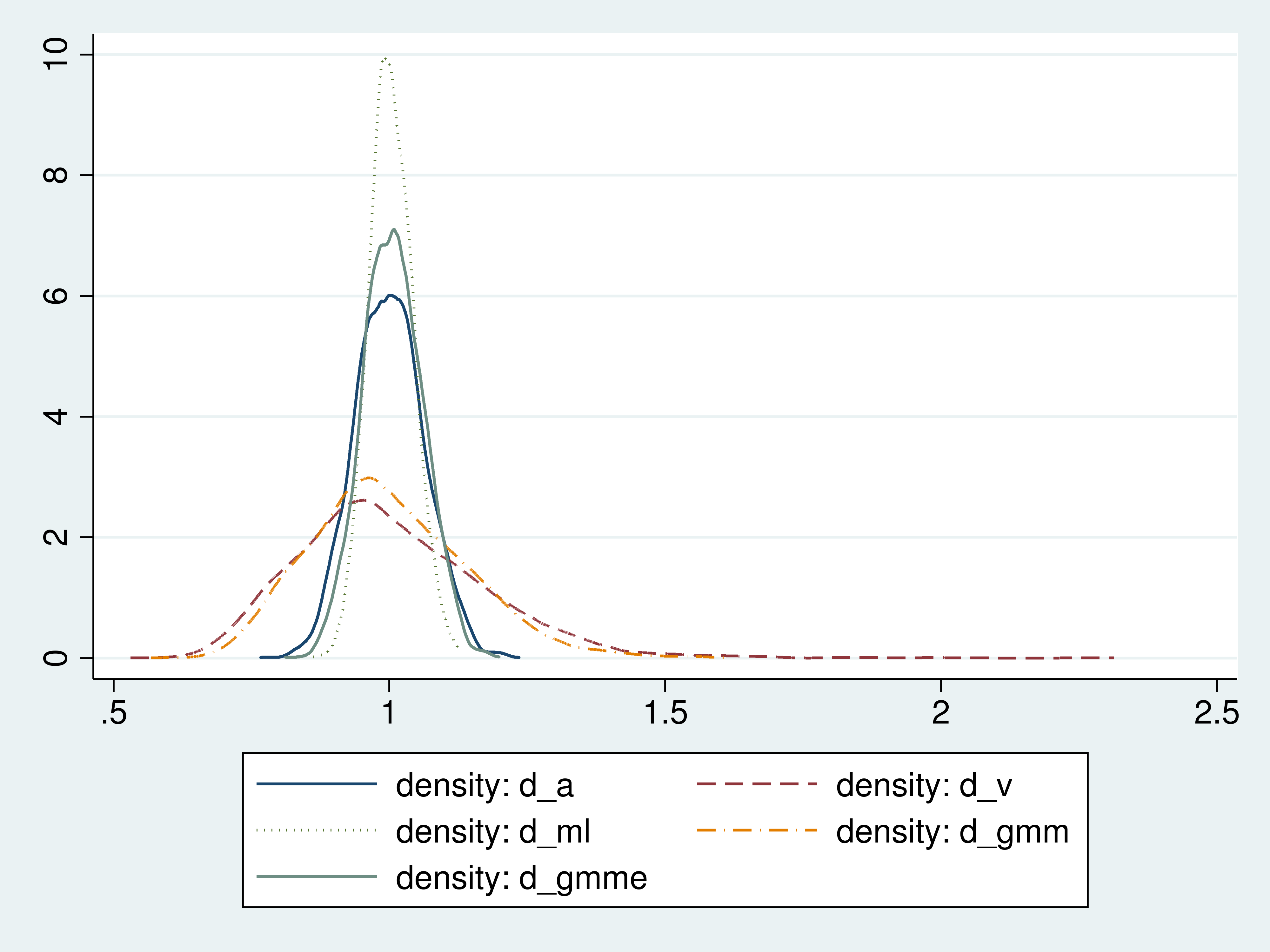
For a greater concept concerning the distributions of those estimators, we graph the densities of their estimates.
Determine 1: Densities of the estimators
The density plots illustrate the effectivity rating that we discovered from the usual deviations of the estimates.
The uniformly weighted GMM estimator is much less environment friendly than the pattern common as a result of it locations the identical weight on the pattern common as on the a lot much less environment friendly estimator based mostly on the pattern variance.
In every of the overidentified circumstances, the GMM estimator makes use of a weighted common of two pattern second circumstances to estimate the imply. The primary pattern second situation is the pattern common. The second second situation is the pattern variance. Because the Monte Carlo outcomes confirmed, the pattern variance gives a a lot much less environment friendly estimator for the imply than the pattern common.
The GMM estimator that locations equal weights on the environment friendly and the inefficient estimator is far much less environment friendly than a GMM estimator that locations a lot much less weight on the much less environment friendly estimator.
We show the burden matrix from our optimum GMM estimator to see how the pattern moments have been weighted.
. quietly gmm ( y - {d}) ( (y-{d})^2 - 2*{d})  , devices( ) winitial(I)

. matlist e(W), border(rows)

-------------------------------------
             | 1         | 2
             |     _cons |     _cons
-------------+-----------+-----------
1            |           |
       _cons |  1.621476 |
-------------+-----------+-----------
2            |           |
       _cons | -.2610053 |  .0707775
-------------------------------------
The diagonal parts present that the sample-mean second situation receives extra weight than the much less environment friendly sample-variance second situation.
Carried out and undone
We used a easy instance for example how GMM exploits having extra equations than parameters to acquire a extra environment friendly estimator. We additionally illustrated that optimally weighting the totally different moments gives necessary effectivity features over an estimator that uniformly weights the second circumstances.
Our cursory introduction to GMM is greatest supplemented with a extra formal remedy just like the one in Cameron and Trivedi (2005) or Wooldridge (2010).
Graph code appendix
use efcomp
native N = _N
kdensity d_a,     n(`N') generate(x_a    den_a)    nograph
kdensity d_v,     n(`N') generate(x_v    den_v)    nograph
kdensity d_ml,    n(`N') generate(x_ml   den_ml)   nograph
kdensity d_gmm,   n(`N') generate(x_gmm  den_gmm)  nograph
kdensity d_gmme,  n(`N') generate(x_gmme den_gmme) nograph
twoway (line den_a x_a,       lpattern(stable))        ///
       (line den_v x_v,       lpattern(sprint))         ///
       (line den_ml x_ml,     lpattern(dot))          ///
       (line den_gmm x_gmm,   lpattern(dash_dot))     ///
       (line den_gmme x_gmme, lpattern(shordash))
References
Cameron, A. C., and P. Ok. Trivedi. 2005. Microeconometrics: Strategies and purposes. Cambridge: Cambridge College Press.
Wooldridge, J. M. 2001. Purposes of generalized technique of moments estimation. Journal of Financial Views 15(4): 87-100.
Wooldridge, J. M. 2010. Econometric Evaluation of Cross Part and Panel Information. 2nd ed. Cambridge, Massachusetts: MIT Press.